Numerical Methods -- Solution of a non-linear algebraic equation -- Module 5

---

Index

1. 1. The Bisection Method
2. 2. Regula-Falsi Method (False position method)
3. 3. Newton-Raphson Method

---

1. The Bisection Method

https://www.youtube.com/watch?v=3j0c_FhOt5U&list=PLU6SqdYcYsfLrTna7UuaVfGZYkNo0cpVC&index=17

The bisection method is a bracketing method that works on continuous functions where you know an interval $[a,b]$ such that $f(a)$ and $f(b)$ have opposite signs (i.e. $f(a)\cdot f(b)<0$. By the Intermediate Value Theorem, there is at least one root in that interval.

So in simple terms it’s an iterative method, where we keep on updating the intervals in every iteration till we get a close to accurate approximation of the real root.

---

Algorithm

1. Initial Bracket: Choose $a$ and $b$ so that $f(a)\cdot f(b)<0$.

2. Midpoint: Compute the midpoint $c=\frac{a+b}{2}$​.

3. Test Sign:

   • If $f(c)=0$ (or is close enough to zero), then $c$ is the root.

   • If $f(a)\cdot f(c)<0$, set $b=c$; otherwise, set $a=c$.

4. Repeat: Continue the process until the interval $[a,b]$ is sufficiently small or until the error is less than a predetermined tolerance.

Note that this is quite a lengthy method and usually takes about 10-15 iterations to get quite close to the real root.

---

Example 1:

So firstly, we need to select two intervals, such that their values should be of opposite signs.

So in Iteration 1:

Let’s go with $1,-1$.

$f(1)=1-1-1=-1$

$f(-1)=-1+1-1=-1$

Both of them are the same.

Let’s try $f(0)$ to see if we get a different result or not :

$f(0)=0-0-1=-1$

Still the same.

Let’s try $f(2)$ then :

$f(2)=8-2-1=5$

So we have :

$f(1)=-1,f(2)=5$

So :

$a=1,b=2$

Now we compute the midpoint $c$ :

$\frac{1+2}{2}=1.5$

Now :

$f(1.5)=0.875$

Since $f(c)>0$ but not quite close enough to $0$, we set $a=c$.

Let’s also maintain a table of values while we are at it:

So far we have had :

Iteration	a	b	midpoint (c)	f(c)
1	1	2	1.5	0.875

Now let’s proceed to iteration 2:

$f(a)\cdot f(c)=-0.875<0$

So we set $b=c$

Iteration	a	b	midpoint (c)	f(c)
1	1	2	1.5	0.875
2	1	1.5	1.25	-0.296

Now let’s proceed to iteration 3:

$f(a)\cdot f(c)=0.296>0$

So we set $a=c$

Iteration	a	b	midpoint (c)	f(c)
1	1	2	1.5	0.875
2	1	1.5	1.25	-0.296
3	1.25	1.5	1.375	0.224

Now, for iteration 4:

$f(a)\cdot f(c)=-0.224<0$

So we set $b=c$

Iteration	a	b	midpoint (c)	f(c)
1	1	2	1.5	0.875
2	1	1.5	1.25	-0.296
3	1.25	1.5	1.375	0.224
4	1.25	1.375	1.3125	-0.051

Now for iteration 5:

$f(a)\cdot f(c)=0.051>0$

So we set $a=c$

Iteration	a	b	midpoint (c)	f(c)
1	1	2	1.5	0.875
2	1	1.5	1.25	-0.296
3	1.25	1.5	1.375	0.224
4	1.25	1.375	1.3125	-0.051
5	1.3125	1.375	1.34375	0.082

For iteration 6:

$f(a)\cdot f(c)=-0.082<0$

So we set $b=c$

Iteration	a	b	midpoint (c)	f(c)
1	1	2	1.5	0.875
2	1	1.5	1.25	-0.296
3	1.25	1.5	1.375	0.224
4	1.25	1.375	1.3125	-0.051
5	1.3125	1.375	1.34375	0.082
6	1.3125	1.34375	1.328125	0.001

So, for iteration 7 :

$f(a)\cdot f(c)=-0.001<0$

So we set $b=c$

Iteration	a	b	midpoint (c)	f(c)
1	1	2	1.5	0.875
2	1	1.5	1.25	-0.296
3	1.25	1.5	1.375	0.224
4	1.25	1.375	1.3125	-0.051
5	1.3125	1.375	1.34375	0.082
6	1.3125	1.34375	1.328125	0.001
7	1.3125	1.328125	1.3203125	-0.018

So for iteration 8:

$f(a)\cdot f(c)=0.018>0$

So we set $a=c$

Iteration	a	b	midpoint (c)	f(c)
1	1	2	1.5	0.875
2	1	1.5	1.25	-0.296
3	1.25	1.5	1.375	0.224
4	1.25	1.375	1.3125	-0.051
5	1.3125	1.375	1.34375	0.082
6	1.3125	1.34375	1.328125	0.001
7	1.3125	1.328125	1.3203125	-0.018
8	1.3203125	1.328125	1.32421875	-2.127

For iteration 9:

$f(a)\cdot f(c)=-2.127<0$

So we set $b=c$

Iteration	a	b	midpoint (c)	f(c)
1	1	2	1.5	0.875
2	1	1.5	1.25	-0.296
3	1.25	1.5	1.375	0.224
4	1.25	1.375	1.3125	-0.051
5	1.3125	1.375	1.34375	0.082
6	1.3125	1.34375	1.328125	0.001
7	1.3125	1.328125	1.3203125	-0.018
8	1.3203125	1.328125	1.32421875	-2.127
9	1.3203125	1.32421875	1.322265625	-0.010

For iteration 10:

$f(a)\cdot f(c)=0.010>0$

So we set $a=c$

Iteration	a	b	midpoint (c)	f(c)
1	1	2	1.5	0.875
2	1	1.5	1.25	-0.296
3	1.25	1.5	1.375	0.224
4	1.25	1.375	1.3125	-0.051
5	1.3125	1.375	1.34375	0.082
6	1.3125	1.34375	1.328125	0.001
7	1.3125	1.328125	1.3203125	-0.018
8	1.3203125	1.328125	1.32421875	-2.127
9	1.3203125	1.32421875	1.322265625	-0.010
10	1.322265625	1.32421875	1.3232422188	-6.284

For the next 5 iterations :

Iteration	a	b	midpoint (c)	f(c)
1	1	2	1.5	0.875
2	1	1.5	1.25	-0.296
3	1.25	1.5	1.375	0.224
4	1.25	1.375	1.3125	-0.051
5	1.3125	1.375	1.34375	0.082
6	1.3125	1.34375	1.328125	0.001
7	1.3125	1.328125	1.3203125	-0.018
8	1.3203125	1.328125	1.32421875	-2.127
9	1.3203125	1.32421875	1.322265625	-0.010
10	1.322265625	1.32421875	1.3232422188	-6.284
11	1.3232422188	1.32421875	1.3237304844	-0.004
12	1.3237304844	1.32421875	1.3239746172	-0.003
13	1.3239746172	1.32421875	1.3240966836	-0.002
14	1.3240966836	1.32421875	1.3241577168	-0.002
15	1.3241577168	1.32421875	1.3241882334	-0.002

Now the question is, which should be the real root?

The condition was :

• If $f(c)=0$ (or is close enough to zero), then $c$ is the root.

Now if we want a really, really precise answer then we can simply opt for $c$ on the 15th iteration, since $f(c)=-0.002$ which is very close to $0$.

Or if we want a good enough root, my personal preference would be the one in iteration 6, since $f(c)=0.001$ is also vey close to $0$ and moreover it’s positive.

So, it all depends on how much precision is asked of us. If we need a more precise answer we can continue iterating to get as close to zero as possible, but I don’t think that further iterations will get much closer than what we already have achieved.

So, the most precise real root is : $1.3241882334$ .

or

The more suitable real root for further calculations would be : $1.328125$ .

This example in the video wasn’t followed into that much depth as I did, however the example after this in the video is covered to much more depth about 15 iterations or so, however since this method is so time consuming, I am not doing this for now.

---

2. Regula-Falsi Method (False position method)

https://www.youtube.com/watch?v=FliKUWUVrEI&list=PLU6SqdYcYsfLrTna7UuaVfGZYkNo0cpVC&index=14

Regula Falsi is also a bracketing method like bisection. However, instead of using the midpoint, it uses a linear interpolation between the endpoints to guess a root. It typically converges faster than the bisection method if the function is nearly linear on the interval.

---

Algorithm

We start off similar to how we do in the Bisection Method

1. Initial Bracket: As with bisection, choose $a$ and $b$ so that $f(a)\cdot f(b)<0$, that is, $a$ and $b$ should have opposite signs.
2. Interpolation: Compute the new estimate using the formula:

$c=\frac{(a\cdot f(b))-(b\cdot f(a))}{f(b)-f(a)}$

3. Test sign:
   • If $f(c)=0$ (or is close enough to zero), then $c$ is the root.
   • Otherwise, if $f(a)\cdot f(c)<0$, set $b=c$, else set $a=c$

---

Example 1

Let’s try with (1, -1)

$f(1)=1-2-5=-4$ $f(-1)=-1-2-5=-8$

Well that didn’t work.

Let’s try with $f(2)$

$f(2)=8-4-5=-1$

Still the same sign. Let’s try with $f(3)$

$f(3)=27-6-5=16$

Now we have something of the opposite sign.

So we have $a=2$ and $b=3$.

Now we can proceed with the interpolation.

This needs to happen for 4 iterations, so we will maintain a table as well.

So, for iteration 1.

$c=\frac{(2\cdot 16)-3\cdot (-1)}{16+1}$

$⟹c=\frac{35}{17}$

$⟹c=2.058$

Iteration	a	b	interpolated value (c)	f(c)
1	2	3	2.0588235294117645	-0.390

Now for iteration 2:

Since $f(a).f(c)>0$, $a=c$

Iteration	a	b	interpolated value (c)	f(c)
1	2	3	2.0588235294117645	-0.390
2	2.058823529	3	2.0812636598450225	-0.147

The values of $c$ and $f(c)$ are all taken out from a very precise calculator, so I will skip the calculations here since I already showed it in iteration 1.

So, for the remaining iterations :

Iteration	a	b	interpolated value (c)	f(c)
1	2	3	2.0588235294117645	-0.390
2	2.0588235294117645	3	2.0812636598450225	-0.147
3	2.0812636598450225 ($f(a).f(c)>0$)	3	2.089639210090847	-0.054
4	2.089639210090847 ($f(a).f(c)>0$)	3	2.0927395743180055	-0.020

So in iteration 4 we see that $f(c)=-0.020$ which is very close to $0$.

So we can accept the real root as $2.0927395743180055$ which is very precise.

Or just, $2.0927$ .

---

Example 2.

Let’s try with a known example of ours to see if we can get almost the same precision in a lesser amount of time.

From our Bisection Method section.

We had chosen the most precise answer after 15 iterations as the real root, which was : $1.3241882334$.

Let’s see if the Regula-Falsi method can arrive at this answer in a much lesser amount of iterations.

So we had chosen : $a=1,b=2$

Let’s run this for 5 iterations.

Instead of doing the calculation by hand this time (I will leave that to you guys as a fun exercise), I will instead use a python script that I cooked up to save myself the time as well.

Here is the code in-case you are tired of using the scientific calculator every time as well.

from collections import defaultdict
 
  
 
# write the equation.
 
  
 
# The function f(x) = x^3 - 2x - 5 # adjust as needed
 
  
 
## default starting values.
 
  
 
possible_roots = []
 
  
 
def f(x):
 
    return x**3 - 2x - 5 # adjust as needed
 
  
 
data_set = defaultdict(list) # initialize a dictionary of arrays
 
  
  
 
def interpolate(a: float | int , b: float | int) -> float | int:
 
    c = ((a * f(b)) - (b * f(a)))/(f(b) - f(a))
 
    return c
 
  
 
# The regula falsi method
 
  
 
def regula_falsi(a: float | int , b: float | int , max_iter:int) -> float | int:
 
    if (a and b <= 0):
 
        print("Error! Both the intervals cannot be of the same sign!")
 
        return ValueError
 
    for i in range(max_iter):
 
        # run for a set amount of iterations
 
        c = interpolate(a, b)
 
  
 
        array = [i+1, a, b, c, f(c)]
 
  
 
        data_set[i].append(array)
 
  
 
        if (f(a) * f(c) < 0):
 
            b = c
 
        else:
 
            a = c
 
  
  
  
 
regula_falsi(1, 2, 10)
 
  
 
for j in range(len(data_set)):
 
    print(data_set[j])
 
  
 
for k in range(len(data_set)):
 
    if abs(data_set[k][0][4]) <= 0.003:
 
        possible_roots.append(data_set[k][0][3])
 
  
 
print("The most precise real root as per the set number of iterations for this equation is: ", possible_roots[-1])

Anyways so here’s the data for 5 iterations.

Iteration	a	b	interpolated value (c)	f(c)
1	1	2	1.1666666666666667	-0.5787037037037035
2	1.1666666666666667 ($f(a).f(c)>0$)	2	1.2531120331950207	-0.2853630296393197
3	1.2531120331950207 ($f(a).f(c)>0$)	2	1.2934374019186834	-0.12954209282197193
4	1.2934374019186834 ($f(a).f(c)>0$)	2	1.3112810214872344	-0.05658848726924948
5	1.3112810214872344 ($f(a).f(c)>0$)	2	1.3112810214872344	-0.024303747183596958

So currently we have $c=1.3112810214872344$ which is very very close to what we obtained from the bisection method for 15 iterations : $1.3241882334$.

Let’s run this for 5 more iterations (don’t do this by hand, since the whole point of Regula-Falsi is to get as close an accurate root as possible in a lesser number of iterations), but since I am quite curious as to where this goes, I will run this for 5 more iterations, so 10 iterations in total

And if you were to see the output here :

 
[[1, 1, 2, 1.1666666666666667, -0.5787037037037035]]
[[2, 1.1666666666666667, 2, 1.2531120331950207, -0.2853630296393197]]
[[3, 1.2531120331950207, 2, 1.2934374019186834, -0.12954209282197193]]
[[4, 1.2934374019186834, 2, 1.3112810214872344, -0.05658848726924948]]
[[5, 1.3112810214872344, 2, 1.3189885035664628, -0.024303747183596958]]
[[6, 1.3189885035664628, 2, 1.322282717465796, -0.010361850069651624]]
[[7, 1.322282717465796, 2, 1.3236842938551607, -0.004403949880785518]]
[[8, 1.3236842938551607, 2, 1.3242794617319507, -0.001869258374370908]]
[[9, 1.3242794617319507, 2, 1.3245319865800917, -0.000792959193252063]]
[[10, 1.3245319865800917, 2, 1.3246390933080368, -0.0003363010300598823]]
 
The most precise real root as per the set number of iterations for this equation is:  1.3246390933080368

We can see that iteration 8 we get the first three decimal places the same as the one obtained from bisection method. And the program considers the most accurate real root as the one in iteration 10, which is $1.3246390933080368$, (since ($f(c)=-0.0003$, which is incredibly close to $0$)) which is even more accurate than the one we obtained after 15 iterations in the Bisection method.

---

3. Newton-Raphson Method

Concept

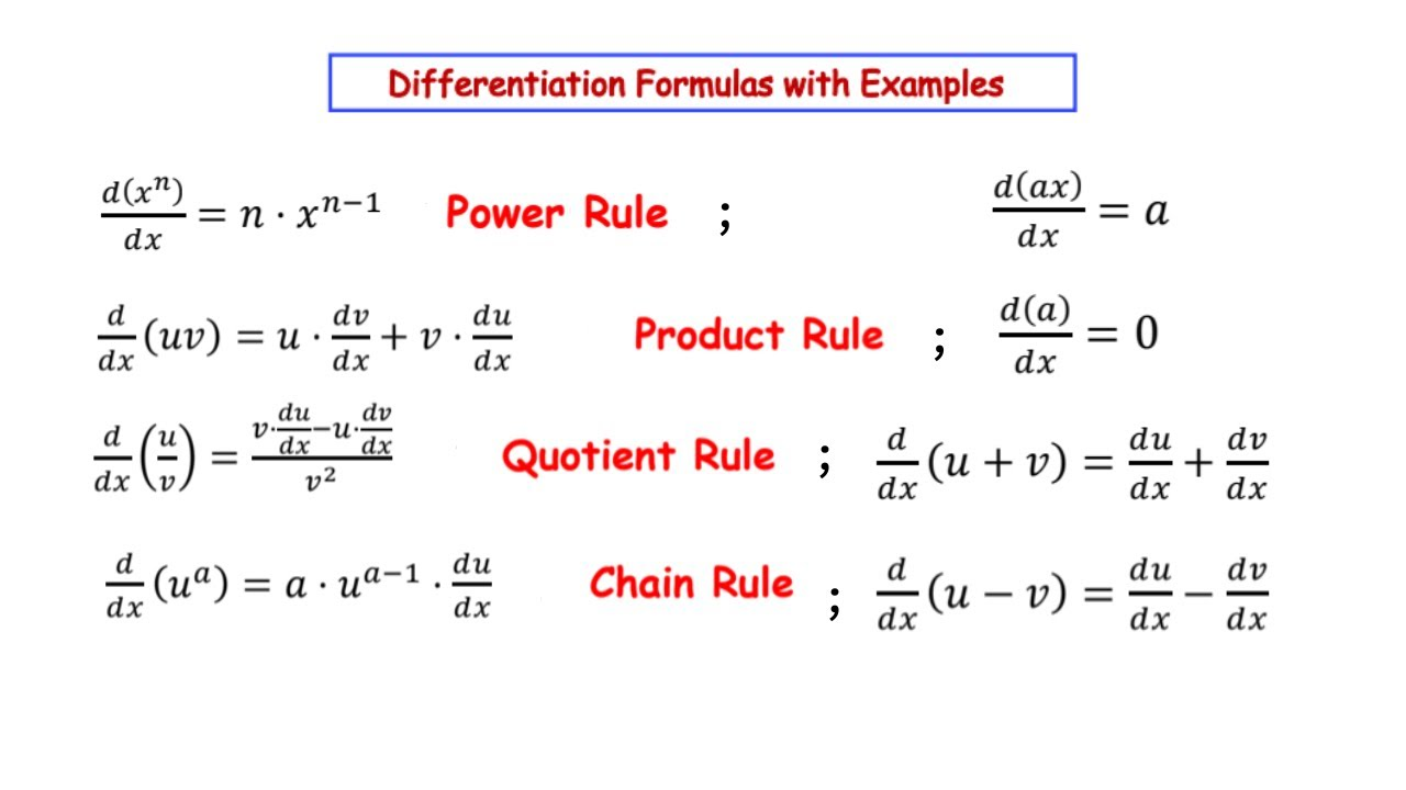
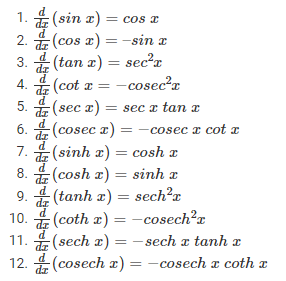
The Newton-Raphson method uses the function’s derivative to find successively better approximations of a root. It requires that the function be differentiable.

The advantage of the Newton-Raphson method is that it’s convergence rate is much faster than the previous two methods mentioned, so we can find the real root in a much less number of iterations.

---

Algorithm

1. Initial Guess: Start with an initial guess $x_0$​.

2. Iteration: Compute the next approximation using:

   $x_{n+1}=x_n-\frac{f(x_n)}{f^{\prime }(x_n)}$​

3. Repeat: Continue until $|x_{n+1}-x_n|$ is less than a predetermined tolerance.

---

Pre-requisites before using this method.

1. Must know differential calculus.

That’s all we will need for the example types of this method.

---

Example 1

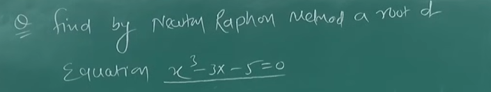
We will run this for 4 iterations

So we have this equation:

$f(x_n)=x^3-3x-5=0$

Let’s try with two initial values :

$f(2)=8-6-5=-3$ $f(3)=27-9-5=13$

So now we will choose $x_0$ as the value which is closest to $0$.

In this case, since $f(2)=-3$, so $x_0=2$.

In the event that both the initial guesses have the same value (opposite sign or not), we can choose either one for $x_0$.

Now let’s find out $f^{\prime }(x_n)$ .

So $f^{\prime }(x_n)=3x^2-3$

So keeping $n=0$.

$x_1=x_0-\frac{f(x_0)}{f^{\prime }(x_0)}$

$⟹x_1=2-\frac{-3}{9}=2+\frac{1}{3}$

$⟹x_1=2+0.3333=2.3333$

Now for $n=1$.

$x_2=x_1-\frac{f(x_1)}{f^{\prime }(x_1)}$

$⟹x_2=2.3333-\frac{0.703}{13.332}$

$⟹x_2=2.2805$

Now for $n=2$

$x_3=x_2-\frac{f(x_2)}{f^{\prime }(x_2)}$

$⟹x_3=2.2805+\frac{1.5548}{4.2522}$

$⟹x_3=2.27902$

Now for $n=3$

$x_4=x_3-\frac{f(x_3)}{f^{\prime }(x_3)}$

$⟹x_4=2.279018$

And lastly for $n=4$

$x_5=x_4-\frac{f(x_4)}{f^{\prime }(x_4)}$

$⟹x_5=2.279018$

And since the value has started to repeat now, we will stop the process, and our real root will be :

$2.279018$

---

Example 2

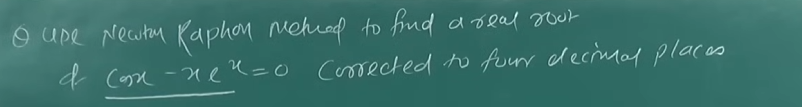
So we have this equation :

$cos(x)-x\cdot e^x=0$

The derivative will be :

$-x{e}^x-e^x-sin(x)$

$=-sin(x)-e^x(x+1)$

In the video $x_0$ was chosen to be 0.5 as the midpoint between $f(0)=1$ and $f(1)=-2.1777$

So if we proceed with that :

For $n=0$

$x_1=0.5-\frac{0.0532}{-2.9525}$

$⟹x_1=0.51802$

For $n=1$

$x_2=0.51802-\frac{-0.0007}{-3.0434}$

$⟹x_2=0.51802-\frac{0.0007}{3.0434}$

$⟹x_2=0.51775$

And this value just keeps on repeating on and on, so this will the real root.

[[0, 0.5, 0.5180260092609312]]
[[1, 0.5180260092609312, 0.5177574240955775]] 
[[2, 0.5177574240955775, 0.5177573636824614]] 
[[3, 0.5177573636824614, 0.5177573636824583]] 
[[4, 0.5177573636824583, 0.5177573636824583]] 
[[5, 0.5177573636824583, 0.5177573636824583]] 
[[6, 0.5177573636824583, 0.5177573636824583]] 
[[7, 0.5177573636824583, 0.5177573636824583]] 
[[8, 0.5177573636824583, 0.5177573636824583]] 
[[9, 0.5177573636824583, 0.5177573636824583]] 
[[10, 0.5177573636824583, 0.5177573636824583]]
[[11, 0.5177573636824583, 0.5177573636824583]]
[[12, 0.5177573636824583, 0.5177573636824583]]
[[13, 0.5177573636824583, 0.5177573636824583]]
[[14, 0.5177573636824583, 0.5177573636824583]]
[[15, 0.5177573636824583, 0.5177573636824583]]
[[16, 0.5177573636824583, 0.5177573636824583]]
[[17, 0.5177573636824583, 0.5177573636824583]]
[[18, 0.5177573636824583, 0.5177573636824583]]
[[19, 0.5177573636824583, 0.5177573636824583]]

As you can see I ran this for 19 iterations to end up with the same value, so the real root is

$0.51775$

However in the question the root has was achieved in the second iteration as $0.578$.

And we could clearly see that the instructor was just jotting the values from a book, so it’s not entirely clear to me as well how this root was achieved.

But if we instead set $x_0=2$ .

[[0, 2, 1.341569059301058]]
[[1, 1.341569059301058, 0.8477005569046928]] 
[[2, 0.8477005569046928, 0.5875567471974426]]

We get the value $0.5875$ which was quite close if you ask me.

However even using $x_0=2$, eventually after some iterations we will get back to the root we found earlier :

[[0, 2, np.float64(1.341569059301058)]]
[[1, np.float64(1.341569059301058), np.float64(0.8477005569046928)]] 
[[2, np.float64(0.8477005569046928), np.float64(0.5875567471974426)]]
[[3, np.float64(0.5875567471974426), np.float64(0.5215809684756582)]]
[[4, np.float64(0.5215809684756582), np.float64(0.5177695600061389)]]
[[5, np.float64(0.5177695600061389), np.float64(0.5177573638070064)]]
[[6, np.float64(0.5177573638070064), np.float64(0.5177573636824583)]]
[[7, np.float64(0.5177573636824583), np.float64(0.5177573636824583)]]
[[8, np.float64(0.5177573636824583), np.float64(0.5177573636824583)]]
[[9, np.float64(0.5177573636824583), np.float64(0.5177573636824583)]]
[[10, np.float64(0.5177573636824583), np.float64(0.5177573636824583)]]
[[11, np.float64(0.5177573636824583), np.float64(0.5177573636824583)]]
[[12, np.float64(0.5177573636824583), np.float64(0.5177573636824583)]]
[[13, np.float64(0.5177573636824583), np.float64(0.5177573636824583)]]
[[14, np.float64(0.5177573636824583), np.float64(0.5177573636824583)]]

As you can see, we are back to $0.51775$. So I guess it’s better we stick to our own math.

---

Example 3

Let’s do one last example on this.

So we have our equation as :

$2(x-3)=lo{g}_{10}(x)$

or

$2(x-3)-lo{g}_{10}(x)=0$

At $x=1$

$f(1)=-4$

At $x=2$

$f(2)=-2.301$

At $x=3$

$f(3)=-0.477$

At $x=4$

$f(4)=1.397$

So here we see that the two points 3 and 4 result in values of opposite signs.

Now we will, generally speaking, select the point that is very close to zero, in this case 3.

But some might select 4 as well for ease of calculation, so in that case it’s generally better to select the mid-point between these two points.

So that would be $3.5$.

So setting $x_0=3.5$

For $n=0$

$x_1=3.5-\frac{0.4559}{1.8759}$

$⟹x_1=3.5-0.2430$

$⟹x_1=3.25696$

For $n=1$

$x_2=3.25696-\frac{0.00099}{1.86665}$

$⟹x_2=3.2569-0.00053$

$⟹x_2=3.25636$

For $n=2$

$x_3=3.25636-\frac{-0.000012411}{1.86663}$

$⟹x_3=3.25636+0.00000664907$

$⟹x_3=3.25636664907$

which is the same as in the video.

Plus this root keeps on repeating as well if we run this a few more iterations :

[[0, 3.5, np.float64(3.2569550080527203)]]
[[1, np.float64(3.2569550080527203), np.float64(3.2563666528736497)]]
[[2, np.float64(3.2563666528736497), np.float64(3.256366649076974)]]
[[3, np.float64(3.256366649076974), np.float64(3.256366649076974)]] 
[[4, np.float64(3.256366649076974), np.float64(3.256366649076974)]] 
[[5, np.float64(3.256366649076974), np.float64(3.256366649076974)]] 
[[6, np.float64(3.256366649076974), np.float64(3.256366649076974)]] 
[[7, np.float64(3.256366649076974), np.float64(3.256366649076974)]] 
[[8, np.float64(3.256366649076974), np.float64(3.256366649076974)]] 
[[9, np.float64(3.256366649076974), np.float64(3.256366649076974)]] 

So the real root of this equation is :

$\boxed{3.25636664907}$

---

Here is the code that I made for the newton raphson method

from collections import defaultdict
 
import sympy as smp
 
import numpy as np
 
  
 
# given equation
 
# 2(x-3) = log_10 (x) or 2(x-3) - log_10(x) = 0 or 2x - 6 - log_10(x) = 0 # simplified the equation for the code to use cheaper operations.
 
  
  
 
x = smp.symbols("x")
 
eqn = 2*x - 6 - smp.log(x, 10) # set the equation as needed
 
  
 
f_numeric = smp.lambdify(x, eqn)
 
eqn_derivative = smp.diff(eqn, x)
 
f_deriv_numeric = smp.lambdify(x, eqn_derivative)
 
  
  
 
data_set = defaultdict(list) # default dictionary of arrays
 
  
  
  
 
def f(x) -> float|int:
 
    return f_numeric(x)
 
  
 
def fprime(x) -> float|int:
 
    return f_deriv_numeric(x)
 
  
  
 
def newton_raphson(x_n: int, n: int):
 
    for i in range(n): # run for n iterations
 
        x_n1 = x_n - (f(x_n) / fprime(x_n))
 
        array = [i, x_n, x_n1]
 
        data_set[i].append(array)
 
  
 
        x_n = x_n1 # update the value
 
  
  
  
 
newton_raphson(3.5, 10)
 
  
 
for k in range(len(data_set)):
 
    print(data_set[k])from collections import defaultdict
 
import sympy as smp
 
import numpy as np
 
  
 
# given equation
 
# 2(x-3) = log_10 (x) or 2(x-3) - log_10(x) = 0 or 2x - 6 - log_10(x) = 0 # simplified the equation for the code to use cheaper operations.
 
  
  
 
x = smp.symbols("x")
 
eqn = 2*x - 6 - smp.log(x, 10) # set the equation as needed
 
  
 
f_numeric = smp.lambdify(x, eqn)
 
eqn_derivative = smp.diff(eqn, x)
 
f_deriv_numeric = smp.lambdify(x, eqn_derivative)
 
  
  
 
data_set = defaultdict(list) # default dictionary of arrays
 
  
  
  
 
def f(x) -> float|int:
 
    return f_numeric(x)
 
  
 
def fprime(x) -> float|int:
 
    return f_deriv_numeric(x)
 
  
  
 
def newton_raphson(x_n: int, n: int):
 
    for i in range(n): # run for n iterations
 
        x_n1 = x_n - (f(x_n) / fprime(x_n))
 
        array = [i, x_n, x_n1]
 
        data_set[i].append(array)
 
  
 
        x_n = x_n1 # update the value
 
  
  
  
 
newton_raphson(3.5, 10)
 
  
 
for k in range(len(data_set)):
 
    print(data_set[k])

You need some knowledge of sympy to tweak the equations properly.

---