Numerical Methods -- Solutions to Linear system of Equations -- Module 4

---

Index

1. Gaussian Elimination method to find the solution for a system of linear equations
2. Gauss-Jordan Elimination Method
3. The Matrix Inversion method.
4. Pre-requisites before using this method (must) (skip ahead if you already know these).
5. 1. The Determinant of a 2x2 matrix.
6. 2. Determinant of a 3x3 matrix
7. 3. Transpose of a matrix.
8. 4. Inverse of a 2x2 matrix.
9. 5. Inverse of a 3x3 matrix
10. Method 1 Using Gauss-Jordan Elimination
11. Method 2 Using the method of matrix of minors, co-factors and adjugate matrix.
12. Finding the solution to a system of equations using the matrix inversion method.
13. LU Factorization Method
14. [[#1-finding-u|1. Finding $U$]]
15. [[#2-finding-l|2. Finding $L$]]
16. [[#3-solving-a-system-of-equations-using-forward-and-backward-substitution-of-lu|3. Solving a system of equations using forward and backward substitution of $LU$]]
17. Gauss-Seidel Method

---

Gaussian Elimination method to find the solution for a system of linear equations

This method converts a system of equations into an upper-triangular form (where all entries below the main diagonal are zero) so that you can then solve for the unknowns via back substitution.

https://www.youtube.com/watch?v=eDb6iugi6Uk

Example 1

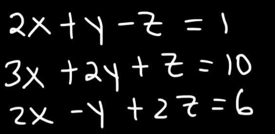
So let’s say we have this system of linear equations here

So first of what we will do is construct an augmented matrix using the coefficients of the equations.

$$\left[\begin{array}{cccc}1& 1& -1& -2\\ 2& -1& 1& 5\\ -1& 2& 2& 1\end{array}\right]$$

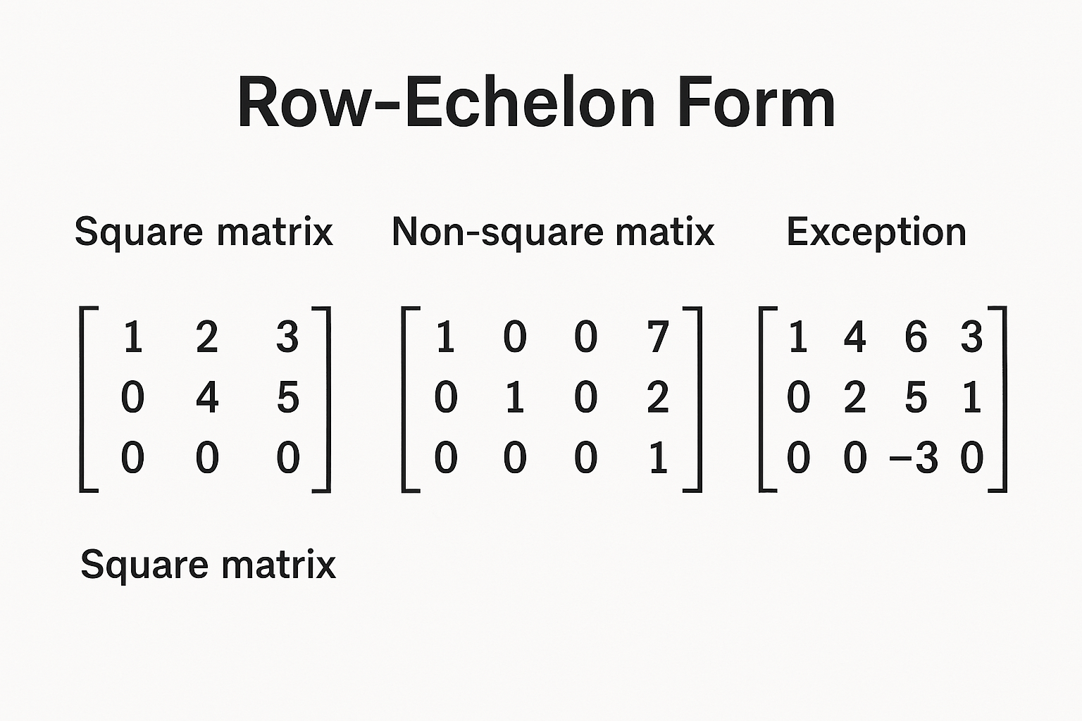
Now what we need to do is to convert this to a row-echelon form.

The row-echelon form of this matrix should be something like this :

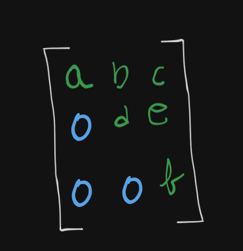
Note that the bottom left half elements below the diagonal line are all zeroes. (Only works for perfect square matrices)

(Image generated by the new version of ChatGPT, not bad indeed.)

So with this matrix, let’s call it $A$

$$\left[\begin{array}{cccc}1& 1& -1& -2\\ 2& -1& 1& 5\\ -1& 2& 2& 1\end{array}\right]$$

How do we convert it to a row-echelon form?

It’s done by doing something called a matrix transformation via matrix row operations.

So first of all we select a pivot element. A pivot element is the first non-zero element we encounter in a matrix.

In $R_1$ we have the first non-zero element as 1. So we select that as the pivot element.

Now all our operations will be centered around $R_1$.

So we can do $R_3\to R_1+R_3$

So the matrix becomes :

$$\left[\begin{array}{cccc}1& 1& -1& -2\\ 2& -1& 1& 5\\ 0& 3& 1& -1\end{array}\right]$$

Remember that when we add two rows, all elements of the rows are affected.

We can then try :

$R_2\to R_2-2R_1$

$$\left[\begin{array}{cccc}1& 1& -1& -2\\ 0& -3& 3& 9\\ 0& 3& 1& -1\end{array}\right]$$

Then we can do :

$R_3\to R_3+R_2$

$$\left[\begin{array}{cccc}1& 1& -1& -2\\ 0& -3& 3& 9\\ 0& 0& 4& 8\end{array}\right]$$

We are already there

This can be done by simply for $R_2$ as:

$R_2\to -\frac{1}{3}\times R_2$

$$\left[\begin{array}{cccc}1& 1& -1& -2\\ 0& 1& -1& -3\\ 0& 0& 4& 8\end{array}\right]$$

We have already reached the row-echelon form, but,

We can further simplify the matrix by performing an operation on $R_3$ :

$R_3\to \frac{1}{4}\times 8$

$$\left[\begin{array}{cccc}1& 1& -1& -2\\ 0& 1& -1& -3\\ 0& 0& 1& 2\end{array}\right]$$

Now we can convert the matrix back to equations as :

$x+y-z=-2$

$y-z=-3$

$z=2$

Now with some simple substitution :

$x+y-2=-2⟹x+y=0⟹x=-y$

Thus :

$y-2=-3⟹y=-3+2⟹y=-1$

Therefore :

$x=-(-1)=1$

So we have the solution for the system of equations as:

$\boxed{x=1;y=-1;z=2}$

Summary:

Always use the format:

$R_{\text{target}}\to R_{\text{target}}-m{R}_{\text{pivot}}$

where :

$m=\frac{Coefficientoftargetx,yorz}{Coefficientofpivotx,yorz}$

For example if we have the rows :

• Pivot Row (Row 1):
  $[21-1\mid 1]$

  Here, if you want to eliminate the $x$-variable, the pivot coefficient is 2.

• Target Row (Row 2):
  $[321\mid 10]$

  The target coefficient for the $x$-variable in Row 2 is $3$.****

---

Example 2

So we can write the matrix as:

$$\left[\begin{array}{cccc}2& 1& -1& 1\\ 3& 2& 1& 10\\ 2& -1& 2& 6\end{array}\right]$$

Here we will select the pivot element as 2.

So all our operations will be centered around $R_1$ for now.

So to solve remove the coefficients of $x$ of $R_2$ and $R_3$ to zero, we will follow the rules mentioned above:

So the target row is $R_3$ and the pivot row is $R_1$.

So $m=\frac{2}{2}=1$

So $R_3\to R_3-m\times R_1⟹R_3\to R_3-\frac{2}{2}\times R_1⟹R_3-R_1$

So

$R_3=[[2-2],[-1-1],[2-(-1)],|6-1]$

$R_3=[0,-2,3|5]$

Therefore the matrix becomes :

$$\left[\begin{array}{cccc}2& 1& -1& 1\\ 3& 2& 1& 10\\ 0& -2& 3& 5\end{array}\right]$$

Now for Row 2, we have :

$m=\frac{3}{2}$

Thus Row 2 will be :

$R_2\to R_2-\frac{3}{2}\times R_1$

$R_2=[[3-\frac{3\times 2}{2}],[2-\frac{3\times 1}{2}],[1-\frac{3\times (-1)}{2}],|10-\frac{3\times 1}{2}]$

$R_2=[0,0.5,2.5|8.5]$

Therefore the matrix now becomes :

$$\left[\begin{array}{cccc}2& 1& -1& 1\\ 0& 0.5& 2.5& 8.5\\ 0& -2& 3& 5\end{array}\right]$$

Now let’s remove the $y$ component of $R_3$ and set it to zero.

So our pivot component for $y$ is $0.5$ in $R_2$.

But why change pivots now?

The reason is that each pivot is used to clear the entries below it in its column. $R_1$​ has already been used to eliminate the $x$-terms in the lower rows. Now, to get the matrix into row-echelon form, the next pivot must appear in a lower row than $R_1$​. In this case, that pivot is in $R_2$​, and it is used to eliminate the $y$-term in $R_3$​.

The way pivots are chosen are that they are taken from a column which hasn’t been used for a pivot, yet.

So :

$m=\frac{-2}{\frac{1}{2}}=-2\times 2=-4$

Therefore $R_3$ will become :

$R_3\to R_3+4R_2$

So $R_3$ will be:

$R_3=[[0+4\times 0],[-2+4\times 0.5],[3+4\times 2.5],|5+4\times 8.5]$

Thus,

$R_3=[0,0,13|39]$

So the matrix will become :

$$\left[\begin{array}{cccc}2& 1& -1& 1\\ 0& 0.5& 2.5& 8.5\\ 0& 0& 13& 39\end{array}\right]$$

Now let’s convert this matrix back to a system of equations :

$2x+y-z=1$

$0.5y+2.5z=8.5$

$13z=39$

So we get :

$z=3$

$0.5y+2.5\times 3=8.5$

$⟹0.5y+7.5=8.5$

$⟹0.5y=1$

$⟹y=\frac{1\times 2}{1}$

$⟹y=2$

And finally :

$2x+2-3=1$

$⟹2x-1=1$

$⟹2x=2$

$⟹x=1$

Thus :

$\boxed{x=1,y=2,z=3}$

---

Gauss-Jordan Elimination Method

This is similar to the previous method, except here we reduce the matrix even further, to something called a “reduced row echelon form”.

https://www.youtube.com/watch?v=eYSASx8_nyg

Now this, is the reduced row echelon form.

where $a,d,f=1$ , essentially resulting in the identity matrix (for square matrices only).

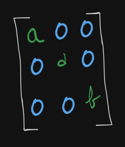
The identity matrix is :

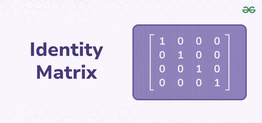
where the diagonal elements of the matrix are 1 and all the other elements are zero.

So let’s say we have this system of equations here:

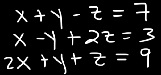
We will solve them in the same manner as we did before, only that there will be a few more operations now.

So let’s convert this system of equations to an augmented matrix first.

$$\left[\begin{array}{cccc}1& 1& -1& 7\\ 1& -1& 2& 3\\ 2& 1& 1& 9\end{array}\right]$$

Let’s set the pivot element to 1 for the $x$ component.

So the target row is $R_2$.

Thus,

$m=\frac{1}{1}=1$

So, $R_2$ will be:

$R_2\to R_2-R_1$

$⟹R_2=[[0],[-2],[3],|-4]$

So the matrix becomes :

$$\left[\begin{array}{cccc}1& 1& -1& 7\\ 0& -2& 3& -4\\ 2& 1& 1& 9\end{array}\right]$$

Now the target is $R_3$. So :

$m=\frac{2}{1}=2$

So:

$R_3\to R_3-m\times R_1$

$⟹R_3=[[2-2],[1-2],[1-2(-1)],|9-14]$

$⟹R_3=[[0],[-1],[3]|-5]$

So the matrix becomes:

$$\left[\begin{array}{cccc}1& 1& -1& 7\\ 0& -2& 3& -4\\ 0& -1& 3& -5\end{array}\right]$$

Now we set the pivot element to -2 for the $y$ component of $R_3$

Thus,

$m=\frac{-1}{-2}=\frac{1}{2}$

So :

$R_3\to R_3-\frac{1}{2}\times R_2$

$⟹R_3=[[0-\frac{1}{2}\times 0],[-1-(\frac{1}{2}\times -2)],[3-(\frac{1}{2}\times 3)]|-5-(\frac{1}{2}\times -4)]$

$⟹R_3=[[0],[0],[1.5]|-3]$

So, the matrix now becomes :

$$\left[\begin{array}{cccc}1& 1& -1& 7\\ 0& -2& 3& -4\\ 0& 0& 1.5& -3\end{array}\right]$$

Now for the $z$ component for $R_2$ , we can set the pivot to 1 of $R_3$. by doing $R_3\to \frac{2}{3}\times R_3$

$$\left[\begin{array}{cccc}1& 1& -1& 7\\ 0& -2& 3& -4\\ 0& 0& 1& -2\end{array}\right]$$

So:

$m=\frac{3}{1}=3$

Note: If we instead tried to set $R_1$‘s -1 as the pivot, it would then affect $R_2$‘s $x$ component while calculation. So it’s better to use a row which won’t be affected in future, that being $R_3$

So,

$R_2\to R_2-3R_3$

$⟹R_2=[0,-2,0|2]$

So, the matrix becomes :

$$\left[\begin{array}{cccc}1& 1& -1& 7\\ 0& -2& 0& 2\\ 0& 0& 1& -2\end{array}\right]$$

Now for $R_1$, :

$m=\frac{1}{-1}=-1$

So :

$R_1\to R_1+R_3$

$⟹R_1=[1,1,0|5]$

Thus the matrix becomes :

$$\left[\begin{array}{cccc}1& 1& 0& 5\\ 0& -2& 0& 2\\ 0& 0& 1& -2\end{array}\right]$$

Now, for the $y$ component of $R_1$, this may seem like that we are going against the rules of selecting a pivot where we can’t reuse an already selected element for a pivot again, but during RREF (reduced row echelon form) there are two types of eliminations :

Forward Elimination vs. Backward Elimination

1. Forward Elimination:

   • Key Point: Once a pivot is chosen in a column, it is used to clear entries downward. You do not worry about entries above because those rows haven’t been processed yet.

     We did this when we were processing the elements below the diagonal line.

2. Backward Elimination (or Back Substitution for RREF):
   Once the matrix is in row-echelon form (all entries below each pivot are zero), you perform backward elimination to clear entries above each pivot. This step ensures that each pivot is the only nonzero entry in its column.

   We are now about to do this with the $y$ component of $R_1$.

   • Why This is Valid:

     • The forward phase ensures that each pivot has zeros below it.

     • The backward phase then uses each pivot to clear above it.

     • Even though the pivot in Row 2 was already used to clear entries below (in Row 3), it must also clear any nonzero entry above it (in Row 1) to satisfy the RREF condition (each pivot column has zeros everywhere except for the pivot itself).

So we can safely select -2 as the pivot.

So :

$m=\frac{1}{-2}$

Before that we scale $R_2$ by $R_2\to -\frac{1}{2}\times R_2$

$$\left[\begin{array}{cccc}1& 1& 0& 5\\ 0& 1& 0& -1\\ 0& 0& 1& -2\end{array}\right]$$

Now $m=1$, (for $R_1$)

So, proceeding with $R_1$ :

$R_1\to R_1-R_2$

$⟹R_1=[1,0,0|6]$

So, the final matrix becomes :

$$\left[\begin{array}{cccc}1& 0& 0& 6\\ 0& 1& 0& -1\\ 0& 0& 1& -2\end{array}\right]$$

Now we can easily convert them back to equations and get the values of $x$, $y$ and $z$.

So,

$x=6$

$y=-1$

$z=-2$

So the solutions are :

$\boxed{x=6,y=-1,z=-2}$

---

The Matrix Inversion method.

Let’s walk through the matrix inversion method step by step. The idea is that if you have a system of linear equations in the form

$Ax=b$

and the coefficient matrix $A$ is invertible (its determinant is nonzero), then the unique solution is given by :

$x=A^{-1}b$

---

Pre-requisites before using this method (must) (skip ahead if you already know these).

1. Knowing how to find out the determinants of 2x2 and 3x3 matrix. (https://www.youtube.com/watch?v=3ROzG6n4yMc)
2. Transpose of a matrix.
3. Knowing how to find the inverses of 2x3 and 3x3 matrix. (https://www.youtube.com/watch?v=aiBgjz5xbyg) (2x2) and (https://www.youtube.com/watch?v=Fg7_mv3izR0) (3x3)

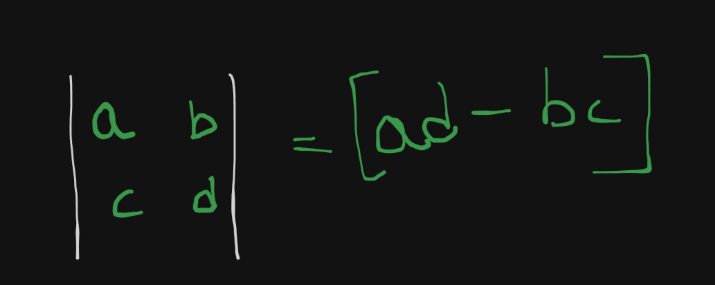
1. The Determinant of a 2x2 matrix.

The determinant of a 2x2 matrix is given by :

Let’s say we have this example :

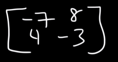
So the determinant of this matrix will be:

$$\det \left|\begin{array}{cc}-7& 8\\ 4& -3\end{array}\right|$$ $$⟹[-7\times -3]-[4\times 8]$$ $$=21-32$$ $$=-11$$

---

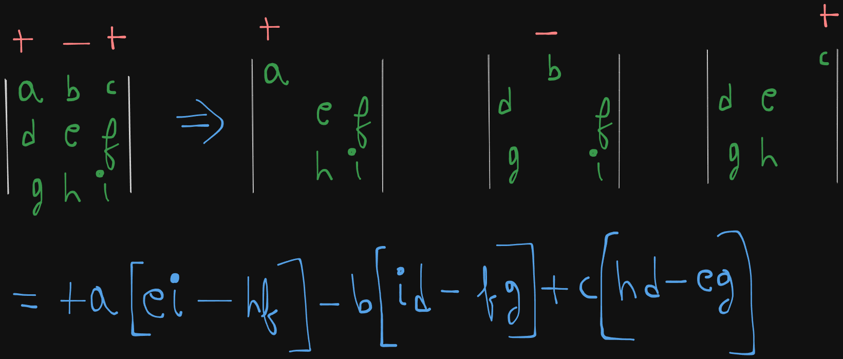
2. Determinant of a 3x3 matrix

Let’s say we have a 3x3 matrix here

$$\left[\begin{array}{ccc}1& 2& 3\\ 4& 5& 6\\ 7& 8& 9\end{array}\right]$$

The determinant is given by :

$$\det \left|\begin{array}{ccc}1& 2& 3\\ 4& 5& 6\\ 7& 8& 9\end{array}\right|$$

which evaluates to :

So let’s say we have this example here :

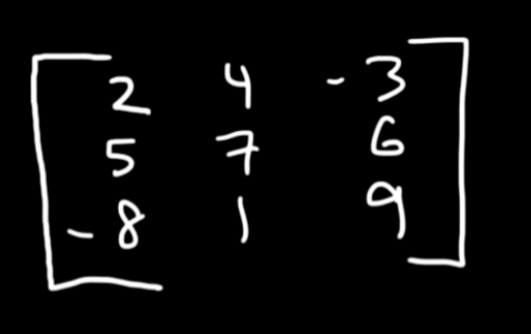
The determinant of this 3x3 matrix will be:

$$\det \left|\begin{array}{ccc}2& 4& -3\\ 5& 7& 6\\ -8& 1& 9\end{array}\right|$$

$⟹+2[(7\times 9)-(1\times 6)]-4[(5\times 9)-(-8\times 6)]+(-3)[(5\times 1)-(-8\times 7)]$

$=+2[57]-4[93]-3[61]$

$=114-372-183$

$-441$

---

3. Transpose of a matrix.

The transpose of a matrix is just it’s rows and columns interchanged.

$$\left[\begin{array}{ccc}1& 2& 3\\ 4& 5& 6\\ 7& 8& 9\end{array}\right]$$

The transpose of this matrix will be :

$$\left[\begin{array}{ccc}1& 4& 7\\ 2& 5& 8\\ 3& 6& 9\end{array}\right]$$

Same for a 2x2 matrix :

$$\left[\begin{array}{cc}a& b\\ c& d\end{array}\right]$$

The transpose will be:

$$\left[\begin{array}{cc}a& c\\ b& d\end{array}\right]$$

---

4. Inverse of a 2x2 matrix.

Note: Before trying to invert a matrix, you must first verify if the matrix is invertible or not. This is done by finding the determinant of the matrix and checking whether it’s zero or not.

If the determinant is zero, the matrix is not invertible, else the matrix is invertible.

So if we have a 2x2 matrix

$$\left[\begin{array}{cc}a& b\\ c& d\end{array}\right]$$

The inverse is given by :

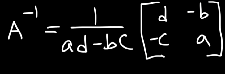
where $\frac{1}{ad-bc}$ is the determinant of the 2x2 matrix.

So let’s say we have this matrix example.

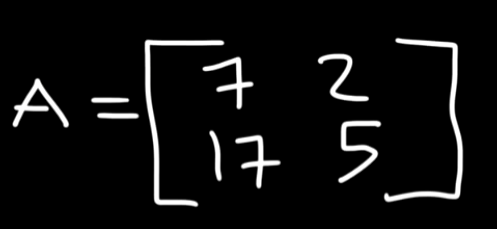
So starting off, let’s find the determinant of this matrix.

$$\det \left|\begin{array}{cc}7& 2\\ 17& 5\end{array}\right|$$

$=[7\times 5]-[17\times 2]$

$=35-34$

$=1$

Now to find the inverse of this matrix :

$$\left[\begin{array}{cc}d& -b\\ -c& a\end{array}\right]$$

or

$$A^{-1}=\left[\begin{array}{cc}5& -2\\ -17& 7\end{array}\right]$$

---

5. Inverse of a 3x3 matrix

Now there are two ways to find the inverse of a 3x3 matrix.

Method 1 : Using Gauss-Jordan Elimination

One way is to use matrix row operations and using the method of Gauss-Jordan elimination to find the inverse of the 3x3 matrix.

https://www.youtube.com/watch?v=Fg7_mv3izR0

So if you have this matrix for example :

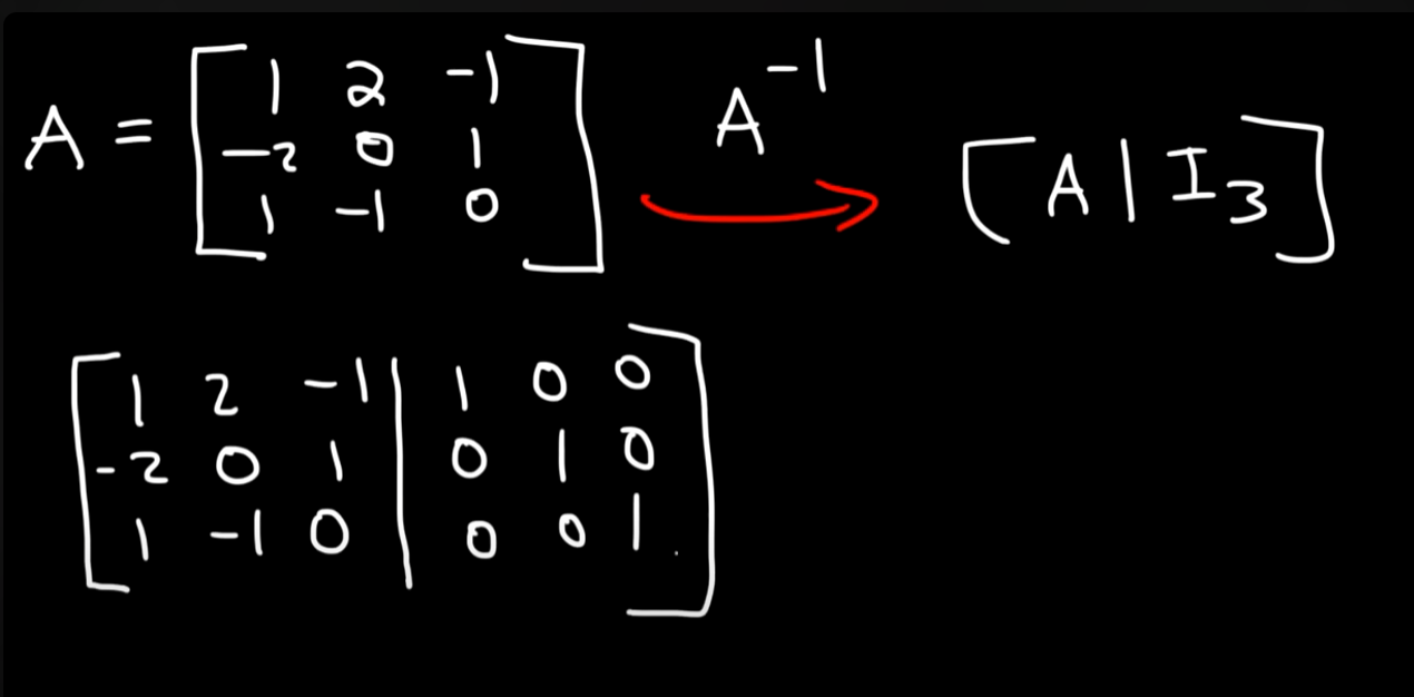
We write it out as in the picture, by augmenting the matrix with the identity matrix.

Then the goal is to perform row operations such that the identity matrix (reduced row echelon form) is on the LHS and on the RHS we get the inverted matrix.

The procedure is the same as Gauss-Jordan elimination, so if you want to see how that’s done you can either watch the video in the link or just scroll up to the section of Gauss-Jordan elimination.

---

Method 2: Using the method of matrix of minors, co-factors and adjugate matrix.

This method is a much less time consuming one that the Gauss-Jordan elimination method.

https://www.khanacademy.org/math/in-in-grade-12-ncert/xd340c21e718214c5:determinants/xd340c21e718214c5:adjoint-and-inverse-of-a-matrix-using-minors-and-cofactors/v/inverting-3x3-part-1-calculating-matrix-of-minors-and-cofactor-matrix

https://www.khanacademy.org/math/in-in-grade-12-ncert/xd340c21e718214c5:determinants/xd340c21e718214c5:adjoint-and-inverse-of-a-matrix-using-minors-and-cofactors/v/inverting-3x3-part-2-determinant-and-adjugate-of-a-matrix

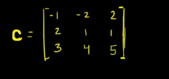
So we start off with a 3x3 matrix

We will create something called a “matrix of minors”.

The matrix of minors is of this format:

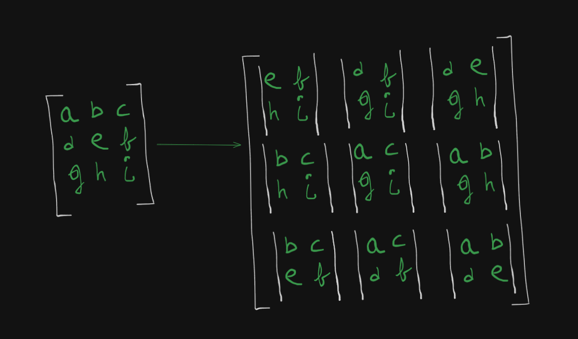
which is basically :

1. Choose an element.
2. Hide the row and column in which that element is.
3. Write the remaining elements in their existing order within a determinant format as singular element of a larger matrix.
4. Keep repeating till all the elements in the original matrix, have been chosen.

So with our example matrix it will be :

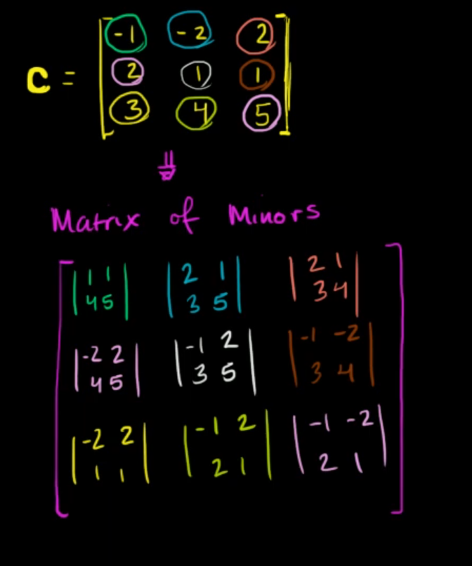
Now after solving the individual determinants :

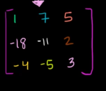
This is the matrix of minors.

Next up is the co-factor matrix.

Simply apply this sign pattern (we see this pattern during the determinant of a 3x3 matrix) :

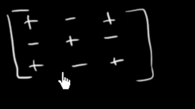
to the elements of the matrix of minors.

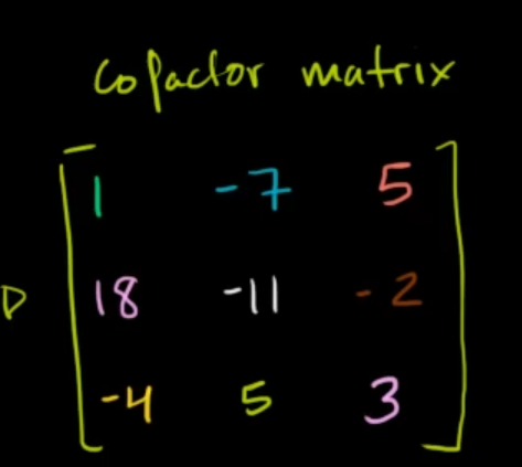
Which now becomes the Co-Factor matrix.

Now we are halfway there!

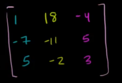
Next up is the adjugate matrix.

The adjugate matrix is just the transpose of the Co-Factor matrix (rows and columns interchanged).

So the final inverse of our 3x3 matrix is the product of the determinant times the adjugate matrix

$A_{3\times 3}^{-1}=\det (A)\times adjugate(A)$

So we already know how to find the determinant of a 3x3 matrix, so I will be skipping that here

The determinant of this matrix is :

So the final inverse is :

which will result in :

---

Finding the solution to a system of equations using the matrix inversion method.

So now that we have all the pre-requisites out of the way we can proceed with the matrix inversion method of finding the solution to a system of equations.

Let’s proceed with the example we used in the Gauss-Jordan elimination method, better to proceed with a known problem as an example.

So we have the system of equations

So let’s convert this system of equations to an augmented matrix first.

$$\left[\begin{array}{cccc}1& 1& -1& 7\\ 1& -1& 2& 3\\ 2& 1& 1& 9\end{array}\right]$$

However here we will do two things.

We split the augmented matrix into two separate matrices.

One will be the coefficient matrix, let’s call it $A$

$$\left[\begin{array}{ccc}1& 1& -1\\ 1& -1& 2\\ 2& 1& 1\end{array}\right]$$

And the variables matrix, let’s call it $\vec{x}$

$$\left[\begin{array}{c}x\\ y\\ z\end{array}\right]$$

And the other one will be the constant matrix, let’s call it $b$:

$$b=\left[\begin{array}{c}7\\ 3\\ 9\end{array}\right]$$

Now we need to find :

$\vec{x}=A^{-1}b$

We will try to invert the coefficient matrix

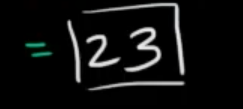
So let’s find out the determinant first:

$\det (A)=+1[-1-2]-1[1-4]+(-1)[1+2]$

$=+1[-3]-1[-3]-1[3]$

$=-3+3-3$

$=-3$

Since $\det (A)\ne 0$ , this means the coefficient matrix is invertible.

So I will proceed with the second method here, as it’s much faster than doing row operations.

Starting with the matrix of minors :

$$\left[\begin{array}{ccc}1& 1& -1\\ 1& -1& 2\\ 2& 1& 1\end{array}\right]$$

will be:

$$\left[\begin{array}{ccc}\left|\begin{array}{cc}-1& 2\\ 1& 1\end{array}\right|& \left|\begin{array}{cc}1& 2\\ 2& 1\end{array}\right|& \left|\begin{array}{cc}1& -1\\ 2& 1\end{array}\right|\\ & & \\ \left|\begin{array}{cc}1& -1\\ 1& 1\end{array}\right|& \left|\begin{array}{cc}1& -1\\ 2& 1\end{array}\right|& \left|\begin{array}{cc}1& 1\\ 2& 1\end{array}\right|\\ & & \\ \left|\begin{array}{cc}1& -1\\ -1& 2\end{array}\right|& \left|\begin{array}{cc}1& -1\\ 1& 2\end{array}\right|& \left|\begin{array}{cc}1& 1\\ 1& -1\end{array}\right|\end{array}\right]$$

(That was quite painful to type and render, but atleast faster than drawing with a mouse).

Now we solve the individual determinants :

$$\left[\begin{array}{ccc}-3& -3& 3\\ 2& 3& -1\\ 1& 3& -2\end{array}\right]$$

So this is the matrix of minors.

Now we apply the sign scheme to get the co-factor matrix:

$$\left[\begin{array}{ccc}-3& 3& 3\\ -2& 3& 1\\ 1& -3& -2\end{array}\right]$$

Now we find the adjugate matrix by transposing the co-factor matrix :

$$\left[\begin{array}{ccc}-3& -2& 1\\ 3& 3& -3\\ 3& 1& -2\end{array}\right]$$

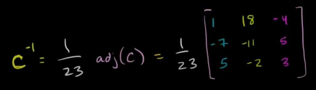
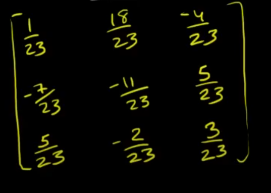
Now we compute the inverse of the matrix :

$$\left[\begin{array}{ccc}-3& -2& 1\\ 3& 3& -3\\ 3& 1& -2\end{array}\right]$$

which will be :

$$\left[\begin{array}{ccc}1& \frac{2}{3}& -\frac{1}{3}\\ -1& -1& 1\\ -1& -\frac{1}{3}& \frac{2}{3}\end{array}\right]$$

Now using the formula :

$\vec{x}=A^{-1}b$

we can find out the value of $x$, $y$ and $z$.

So :

\begin{array}{ccc} x \\ y \\ z \end{array} \right] \ = \ \left[ \begin{array}{ccc} 1 & \frac{2}{3} & -\frac{1}{3} \\ -1 & -1 & 1 \\ -1 & -\frac{1}{3} & \frac{2}{3} \end{array} \right] \ \times \left[ \begin{array}{ccc} 7 \\ 3 \\ 9 \end{array} \right]

For $x$, multiply each element of $b$ to each element of the first row of $A^{-1}$ and add :

$x=7\times 1+\frac{2}{3}\times 3+-\frac{1}{3}\times 9$

$⟹x=7+2-3$

$⟹x=6$

Similarly :

$y=-7-3+9$

$⟹y=-1$

And lastly :

$z=-7-\frac{1}{3}\times 3+\frac{2}{3}\times 9$

$⟹z=-7-1+6$

$⟹z=-2$

So we get a unique solution this time as :

$\boxed{x=6,y=-1,z=-2}$

---

LU Factorization Method

https://www.youtube.com/watch?v=dwu2A3-lTGU&list=PLU6SqdYcYsfLrTna7UuaVfGZYkNo0cpVC&index=20

https://www.youtube.com/watch?v=a9S6MMcqxr4 (A better explanation of how to find the $L$ and $U$ matrices in my opinion ).

https://www.youtube.com/watch?v=Tzrg0GgEfZY (continuation, shows how to find the solution of a system of equations using the $LU$ matrices).

The LU factorization method is an iterative method, that is the solving is carried out in iterations.

LU factorization is especially useful when you need to solve multiple systems with the same coefficient matrix $A$ but different right-hand side vectors $b$, since you factor $A$ only once.

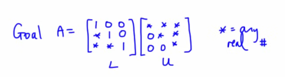
The idea behind LU factorization is to write the coefficient matrix $A$ as the product of a lower triangular matrix $L$ (with 1’s on the diagonal) and an upper triangular matrix $U$:

$A=LU$

Once we have this factorization, we solve the system:

$Ax=b$

by first solving

$Ly=b$

which is forward substitution

and then solving :

$Ux=y$

which is backward substitution

---

So let’s work first on understanding how to find :

$A=LU$

with an example here.

So with this example matrix

(the $\ast =anyrealnumber$)

or

$L=\left[\begin{array}{ccc}1& 0& 0\\ l_{21}& 1& 0\\ l_{31}& l_{32}& 1\end{array}\right]\text{and}U=\left[\begin{array}{ccc}{u}_{11}& u_{12}& u_{13}\\ 0& u_{22}& u_{23}\\ 0& 0& u_{33}\end{array}\right]$

Note that the matrix $U$ is in the row-echelon form.

---

1. Finding $U$

So we start by finding $U$.

That can be done by simply using Gauss elimination method.

$$\left[\begin{array}{ccc}2& 2& 3\\ 5& 9& 10\\ 4& 1& 2\end{array}\right]$$

We set the pivot to $R_1$.

So for $R_2$ :

$m=\frac{5}{2}$

So $R_2\to R_2-\frac{5}{2}{R}_1$ $⟹R_2=[(5-5),(9-5),(10-\frac{15}{2})]$

$⟹R_2=[0,4,\frac{5}{2}]$

So the matrix becomes :

$$\left[\begin{array}{ccc}2& 2& 3\\ 0& 4& \frac{5}{2}\\ 4& 1& 2\end{array}\right]$$

Now for $R_3$

$m=2$

So $R_3=R_3-2R_1$

$$⟹R_3=[(4-4),(1-4),(2-6)]$$

$⟹R_3=[0,-3,-4]$

So the matrix becomes:

$$\left[\begin{array}{ccc}2& 2& 3\\ 0& 4& \frac{5}{2}\\ 0& -3& -4\end{array}\right]$$

Now for the $y$ component of $R_3$, we select 4 as the pivot from $R_2$.

So :

$m=\frac{-3}{4}$

Then :

$R_3=R_3+\frac{3}{4}{R}_2$

$⟹R_3=[0,(-3+3),(-4+\frac{15}{8})]$

$⟹R_3=[0,0,-\frac{17}{8}]$

So the matrix $U$ is :

$$\left[\begin{array}{ccc}2& 2& 3\\ 0& 4& \frac{5}{2}\\ 0& 0& -\frac{17}{8}\end{array}\right]$$

---

2. Finding $L$

Now the matrix $L$ is quite easy to find.

The upper triangular half of $L$ is similar to the identity matrix, where the diagonals are all 1s and the elements above the diagonal line are all zeroes.

Now the lower triangular half, which represents the $L$ matrix, is just the previous $m$ values we used to find $U$, per element in the correct order.

So we currently have $L$ as :

$$\left[\begin{array}{ccc}1& 0& 0\\ & 1& 0\\ & & 1\end{array}\right]$$

Now we will just fill in the gaps using the $m$ values we found in the correct order for $U$.

So, for the $x$ component of $R_2$, $m=\frac{5}{2}$

$$\left[\begin{array}{ccc}1& 0& 0\\ \frac{5}{2}& 1& 0\\ & & 1\end{array}\right]$$

Next, for the $x$ component of $R_3$, $m=2$

$$\left[\begin{array}{ccc}1& 0& 0\\ \frac{5}{2}& 1& 0\\ 2& & 1\end{array}\right]$$

And lastly, for the $y$ component of $R_3$, $m=-\frac{3}{4}$

$$\left[\begin{array}{ccc}1& 0& 0\\ \frac{5}{2}& 1& 0\\ 2& -\frac{3}{4}& 1\end{array}\right]$$

And this the $L$ matrix.

---

3. Solving a system of equations using forward and backward substitution of $LU$

So, now we know how to find :

$A=LU$

Now let’s proceed to solving a system of equations with forward and backward substitution.

Let’s use a new example for this part:

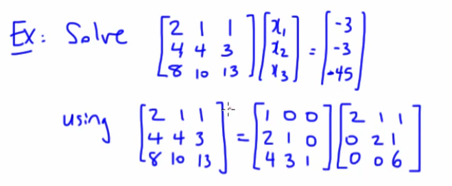
This time we have already been given $L$ and $U$, since we just did a problem to how to find the two matrices.

Now by default we have the system of equations as :

$A\vec{x}=b$

So :

$$\left[\begin{array}{ccc}2& 1& 1\\ 4& 4& 3\\ 8& 10& 13\end{array}\right]$$ $$\vec{x}=\left[\begin{array}{c}x\\ y\\ z\end{array}\right]$$ $$b=\left[\begin{array}{c}-3\\ -3\\ -45\end{array}\right]$$

---

And since $A=LU$.

$$⟹LU\vec{x}=b$$

Now to simplify things, let $U\vec{x}=\vec{y}$

So now we will be solving :

$L\vec{y}=b$

which will look like this :

$$\left[\begin{array}{ccc}{y}_1& y_2& y_3\end{array}\right]=\left[\begin{array}{cccc}1& 0& 0& -3\\ 2& 1& 0& -3\\ 4& 3& 1& -45\end{array}\right]$$

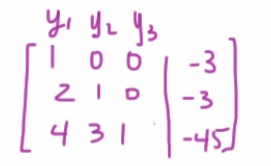
So we will get :

$y_1=-3$

$2y_1+y_2=-3$

$2[-3]+y_2=-3$

$⟹y_2=3$

$4y_1+3y_2+y_3=-45$

$⟹4[-3]+3[3]+y_3=-45$

$⟹-12+9+y_3=-45$

$⟹-3+y_3=-45$

$⟹y_3=-42$

So we have :

$\boxed{y_1=-3,y_2=3,y_3=-42}$

So

$$\left[\begin{array}{c}-3\\ 3\\ -42\end{array}\right]$$

Now we go back to this part that :

$U\vec{x}=\vec{y}$

So we will use this equation to find $\vec{x}$.

Therefore :

$$\left[\begin{array}{ccc}{x}_1& x_2& x_3\end{array}\right]=\left[\begin{array}{ccc}2& 1& 1\\ 0& 2& 1\\ 0& 0& 6\end{array}\right]=\left[\begin{array}{c}-3\\ 3\\ -42\end{array}\right]$$

So :

$6x_3=-42⟹x_3=-7$

$2x_2-7=3$

$⟹2x_2=10$

$x_2=5$

And lastly :

$2x_1+5-7=-3$

$⟹2x_1-2=-3$

$2x_1=-1$

$x_1=-\frac{1}{2}$

So :

$$\vec{x}=\left[\begin{array}{c}-\frac{1}{2}\\ 5\\ -7\end{array}\right]$$

Now since :

$$\vec{x}=\left[\begin{array}{c}x\\ y\\ z\end{array}\right]$$

We have our solution to the system of equations as:

$\boxed{x=-\frac{1}{2},y=5,z=-7}$

---

Example 2

Let’s try out with a known example from our previous sections to see if we can get the same solution or not with the LU factorization method.

So we have these three equations again.

Let’s represent them in the matrix format.

One will be the coefficient matrix, let’s call it $A$

$$\left[\begin{array}{ccc}1& 1& -1\\ 1& -1& 2\\ 2& 1& 1\end{array}\right]$$

And the variables matrix, let’s call it $\vec{x}$

$$\left[\begin{array}{c}x\\ y\\ z\end{array}\right]$$

And the other one will be the constant matrix, let’s call it $b$:

$$b=\left[\begin{array}{c}7\\ 3\\ 9\end{array}\right]$$

---

Step 1. Finding $U$.

We will perform Gauss-elimination on the coefficient matrix to row-echelon form, which will be $U$.

Since this a known matrix which we have used in our previous examples, I will just skip the row-operations part.

$$\left[\begin{array}{ccc}1& 1& -1\\ 0& -2& 3\\ 0& 0& 1.5\end{array}\right]$$

or

$$\left[\begin{array}{ccc}1& 1& -1\\ 0& -2& 3\\ 0& 0& \frac{3}{2}\end{array}\right]$$

Now this is $U$ matrix.

---

Step 2. Finding $L$

The $L$ matrix will just be the $m$ values we used in the correct order to obtain $U$ and the upper triangular half being similar to the identity matrix.

The $m$ values in the correct order are :

1 2 $\frac{1}{2}$

So the $L$ matrix will be :

$$\left[\begin{array}{ccc}1& 0& 0\\ 1& 1& 0\\ 2& \frac{1}{2}& 1\end{array}\right]$$

---

Step 3. Performing forward and backward substitution to solve the system of equations.

Now we set :

$LU\vec{x}=b$

where $U\vec{x}=\vec{y}$

So we will first solve :

$L\vec{y}=b$

So :

$$\left[\begin{array}{ccc}{y}_1& y_2& y_3\end{array}\right]=\left[\begin{array}{cccc}1& 0& 0& 7\\ 1& 1& 0& 3\\ 2& \frac{1}{2}& 1& 9\end{array}\right]$$

$y_1=7$

$y_2=3-7=-4$

$2y_1+\frac{1}{2}{y}_2+y_3=9$

$⟹14-2+y_3=9$

$⟹y_3=-3$

Thus :

$$\vec{y}=\left[\begin{array}{c}7\\ -4\\ -3\end{array}\right]$$

Next we perform back substitution to find :

$U\vec{x}=\vec{y}$

So :

$$\left[\begin{array}{ccc}{x}_1& x_2& x_3\end{array}\right]=\left[\begin{array}{ccc}1& 1& -1\\ 0& -2& 3\\ 0& 0& \frac{3}{2}\end{array}\right]=\left[\begin{array}{c}7\\ -4\\ -3\end{array}\right]$$

So :

$x_3=\frac{2}{3}\times -3=-2$

$-2x_2-6=-4$

$⟹x_2=-1$

$x_1-1+2=7$

$⟹x_1+1=7=6$

Thus, we have :

$$\vec{x}=\left[\begin{array}{c}6\\ -1\\ -2\end{array}\right]$$

Therefore we have the solution to the system of equations as :

$\boxed{x=6,y=-1,z=-2}$

which is the same as the one we found before.

So our answer and this approach to the LU method is correct.

---

Gauss-Seidel Method

The Gauss–Seidel method is an iterative procedure that updates each variable in sequence using the most recent values from the previous updates. The general idea is to rewrite each equation in the form :

$x=f_1(x,y,z),y=f_2(x,y,z),z=f_3(x,y,z)$​

Then, starting from an initial guess, you update one variable at a time in a fixed order.

So we have our system of equations:

A common first step is to solve each equation for a different variable. One way to rearrange is:

1. $x=7-y+z$

2. $y=x+2z-3$

3. $z=9-2x-y$

Now that we have values in terms of all three variables. We can start iterations on this and try to approximate the values of $x$ , $y$ and $z$ as accurately as possible.

Now for the approximation to be as accurate as possible, the system of equations must converge.

For a convergence to take place the system of equations must be diagonally dominant.

We can check whether a system is diagonally dominant or not by creating the coefficient matrix :

$$\left[\begin{array}{ccc}1& 1& -1\\ 1& -1& 2\\ 2& 1& 1\end{array}\right]$$

Now, we can check for diagonal dominance as follows :

• Row 1: $|1|\ge |1|+|-1|=1+1=2$

Here we see that the selected diagonal element is not greater than the sum of the remaining elements in it’s row, so it’s not diagonally dominant.

Similarly :

• Row 2: $|-1|\ge |1|+|2|=3$

Again the selected diagonal element is less than the sum of the remaining elements in it’s row, so it’s not diagonally dominant.

Lastly :

• Row 3: $|1|\ge |2|+|1|=3$ Once again the selected diagonal element is less than the sum of the remaining elements in it’s row, so it’s not diagonally dominant.

Since the matrix is not strictly diagonally dominant, the Gauss–Seidel method may not converge for this system.

---

Anyways, we will start with the iterations to see where it leads us :

Starting initially :

$x^{(k)},y^{(k)},z^{(k)}$

and we assume all three to be zero.

So :

$$x^{(k)}=0,y^{(k)}=0,z^{(k)}=0$$

Now in the first iteration, we get the values of $x,y,andz$ from the equations as :

1. $x^{(k+1)}=7-0+0=7$

2. $y^{(k+1)}=7+2(0)-3=7-3=4$ See that we immediately used the updated value of $x$ in the second iteration while updating $y^{\prime }s$ value.

3. $z^{(k+1)}=9-2(7)-4=9-14-4=-9$

Now in the second iteration :

1. $x^{(k+2)}=7-4-9=-6$

2. $y^{(k+2)}=-6-18-3=-27$

3. $z^{(k+1)}=9+12+27=48$

So let’s do a check to see if the system is converging or diverging.

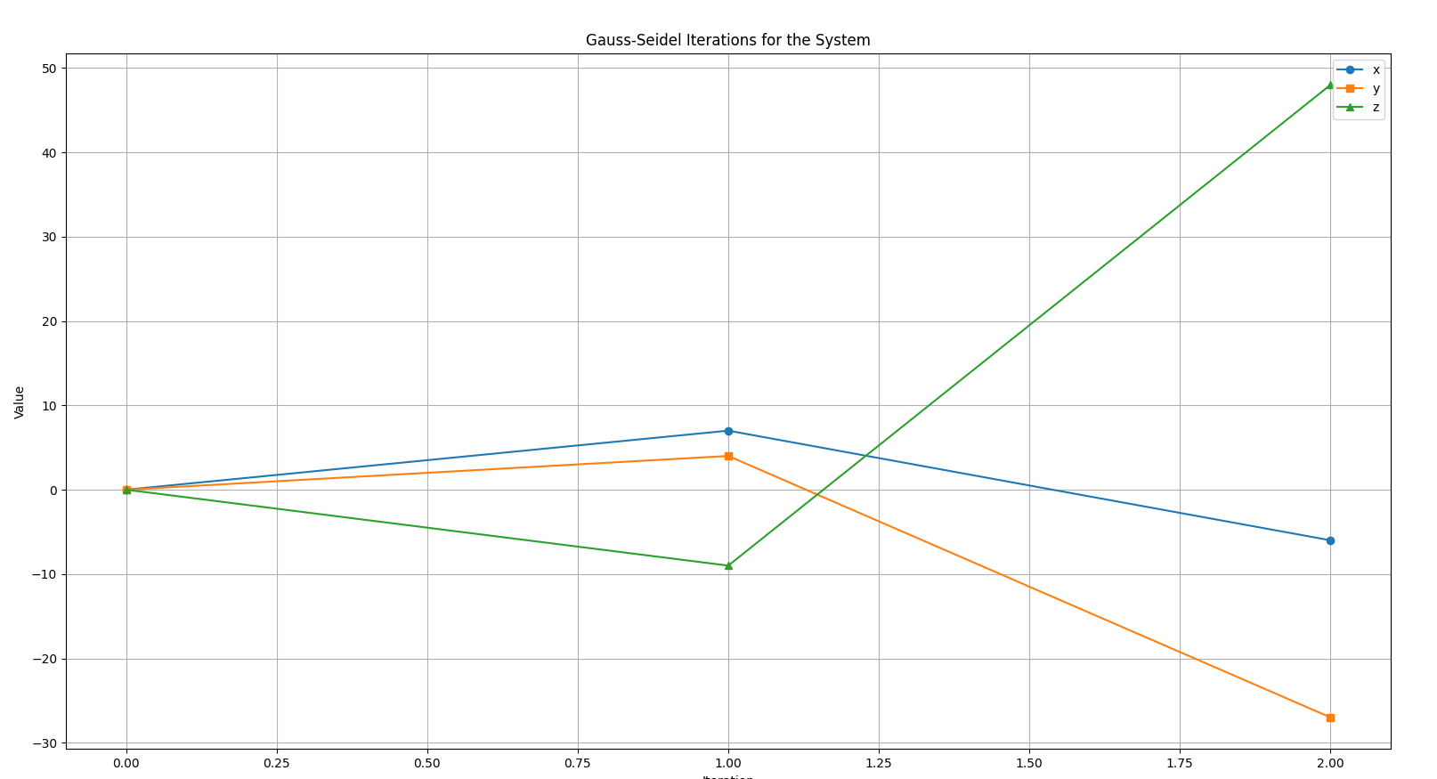
We can already observe that the system is starting to spread out (diverge) at iteration 2 itself, due to a lack of diagonal dominance.

So we can see that in iteration one the system was at :

$(7,4,-3)$

In the second iteration we have the system at :

$(-6,-27,48)$

If we continue for 3 more iterations, let’s see where this leads us.

Iteration 3:

1. $x^{(k+3)}=7+27+48=82$

2. $y^{(k+3)}=82+2(48)-3=175$

3. $z^{(k+3)}=9-2(82)-175=-330$

---

Iteration 4 :

1. $x^{(k+4)}=7-175-330=-498$

2. $y^{(k+4)}=-498-2(330)-3=-1161$

3. $z^{(k+4)}=9+2(498)+1161=2166$

---

Iteration 5:

1. $x^{(k+5)}=7+1161+2166=3334$

2. $y^{(k+5)}=3334+2(2166)-3=7663$

3. $z=9-2(3334)-7663=-14332$

---

So we can see the values have skyrocketed too much due to lack of diagonal dominance and subsequent divergence :

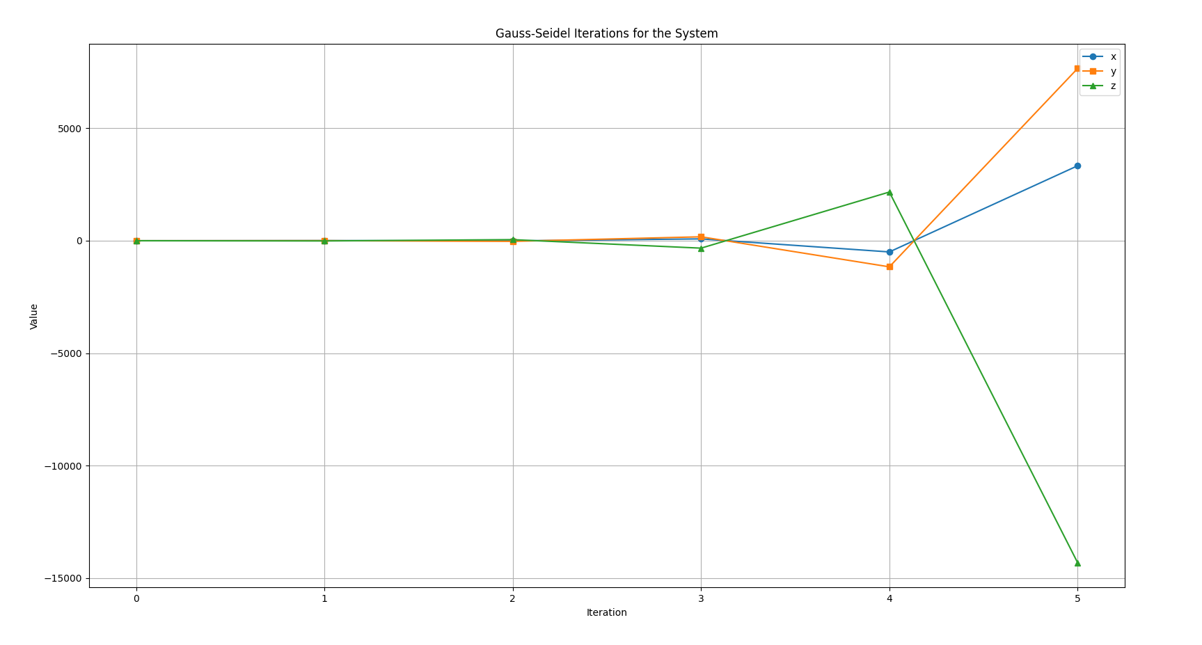
So in this case, the Gauss-Seidel method is not applicable for a system of equations that is not diagonally dominant as it diverges too much from it’s solution :

$\boxed{x=6,y=-1,z=-2}$

https://www.youtube.com/watch?v=gxy6VI1hEfs&list=PLU6SqdYcYsfLrTna7UuaVfGZYkNo0cpVC&index=26

This video has another example that is diagonally dominant, and in that case the Gauss-Seidel method works and we get an accurate approximation after 4-5 iterations, so you can try that example out.

---