Index
- 1. First() and Follow() methods recap
- LL(1) compatibility checking
- LL(1) parsing table creation
- Checking if a grammar is SLR(1) compatible.
- Checking whether a grammar is LALR(1) compatible or not
- Operator Precedence Parsing
FLAT Recap: Regular Grammar and Regular Expressions
FLAT Recap : Context Free Grammar
Index
- Context Free Language
- Derivation Tree
- Reduction/Simplification of Context-Free Grammar
- 1. Reduction of CFG
- 2. Removal of Unit Production
- 3. Removal of Null Productions
- 4. Removal of Left Recursions
1. First() and Follow() methods recap
1. First() method
Recapping the rules
First(terminal variable) = terminal variableFirst(ε) = εPlacing ε in any non-terminal variable will completely rule it out and move to the next non-terminal variable(if any).In case of a non-terminal on the RHS, we find the first of that non-terminal, i.e the first of any non-terminal variable will always contain a terminal variable.
Example 1
S -> A B c
A -> a | b A
B -> d B | ε
So the first(S) would be A.
first(A) = ab
first(B) = dε
So we can say that first(S) becomes ab.
Example 2
S -> ABC
A -> a | b | ε
B -> c | d | ε
C -> e | f | ε
So here we have first(S) = A
first(A) = abε
first(B) = cdε
first(C) = efε
So we can also say that first(S) = abε
Now as soon as ε is placed, A will get ruled out and the next non-terminal is considered, which is B in this case.
So first(S) = abcdε.
Again, in the same way, B is ruled out and now C is considered.
So first(S) = abcdefε. No more non-terminals left to consider so this is the First() set of S.
Example 3
E -> TE'
E' -> *TE'|ε
T -> FT'
T' -> ε | +FT'
F -> id|(ε
first(E) = T
first(T) = F
first(F) = id(
Thus first(E) = id(
2. Follow() method
Recapping the rules
Follow(S) where S is the start symbol = {$}Follow(A) where A is a non-terminal symbol, goes to it's immediate right.In case of a non-terminal variable on the right, we find it's First()In case of ε being present on the right of a non-terminal, it's Follow() will be the Follow(LHS), mostly the Follow(S) where S is the start symbol or {$} or any other non-terminal variable on the LHS.ε is never included in the Follow set.As previously mentioned, applying ε in a non-terminal symbol will rule it out and the next non-terminal symbol will be considered (if any).
Example 1
S -> A B c
	A -> a | b A
B -> d B | ε
we can re-write the grammar as
S -> A B c ε
A -> a ε | b A ε
B -> d B ε | ε
So follow(S) will include $
And follow(A) = first(B)
first(B) = dε
Also from A -> a ε | b A ε , we see that ε maps back to it’s start symbol, which is also A.
So follow of it’s start symbol will be $
Therefore follow(A) = {$, d}
ε was skipped as it is not included in follow sets.
Therefore follow(B) = c and from B -> d B ε | ε, there is ε on the RHS of B so it maps back to the start symbol, which is also B. Now follow of any start symbol is $.
So follow(B) = {$, c}
Example 2
S -> A C B
A -> a A | ε
B -> b B | ε
C -> c C | d
This grammar can be re-written as :
S -> A C B ε
A -> a A ε | ε
B -> b B ε | ε
C -> c C ε | d ε
follow(S) = {$}
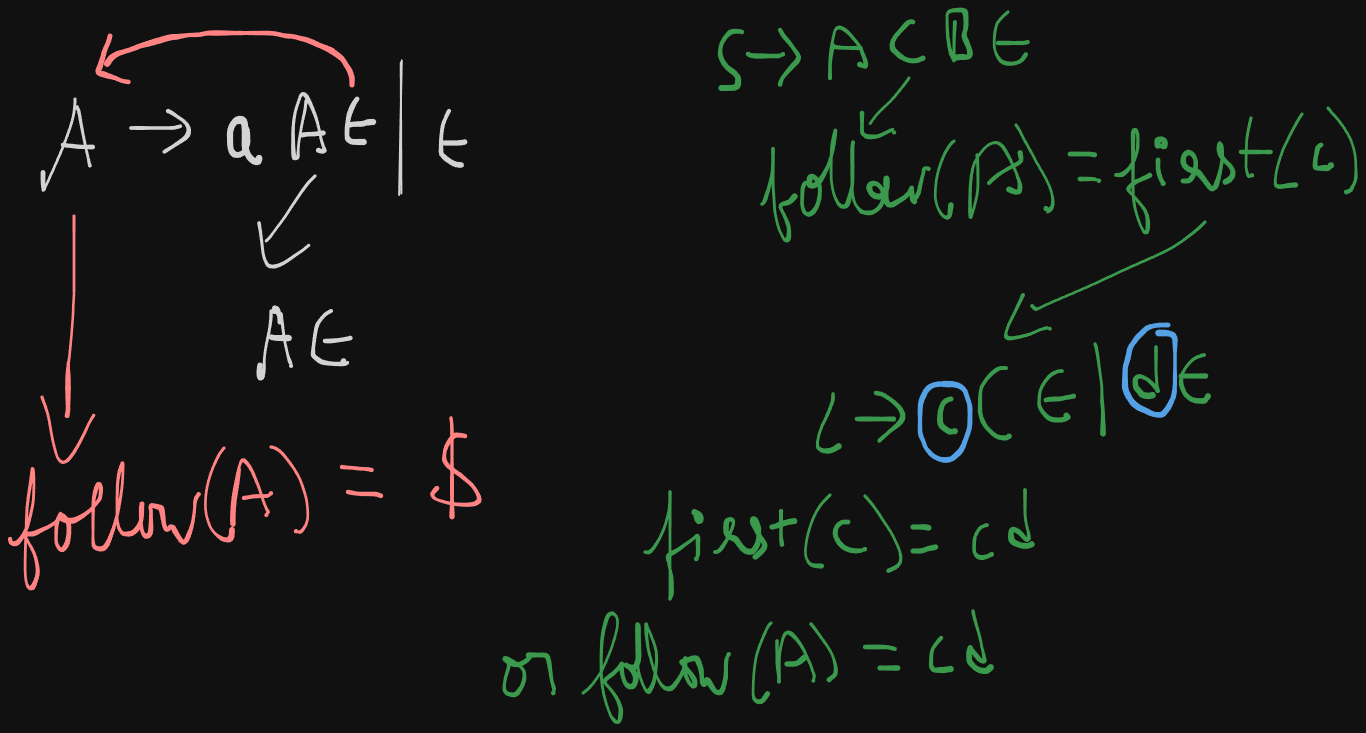
follow(A) = {$, first(C)} = {$, cd}
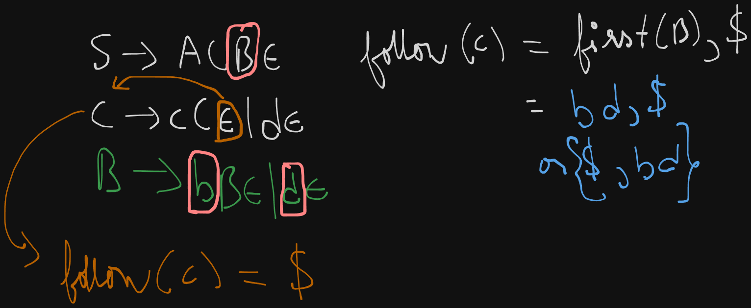
follow(B) = {$}
follow(C) = {$, first(B)} = {$, b}, ε not included
LL(1) compatibility checking
The LL(1) parser belongs to the category of Top-Down parsing.
LL(1) parsing table creation
- Find
first()andfollow()of all variables - Assign numbers to the productions
- Create the parsing table.
- Fill in the values based on the
first()of each variable on RHS of each production - In case of
εon the RHS, we will find thefollow()of the production’s start symbol
Example 1
So let’s say we have been given a grammar
S -> (L) | a
L -> SL'
L' -> ε | ,SL'
This grammar can be re-written as:
S -> (L)ε | aε
L -> SLε'
L' -> ε | ,SL'ε
First sets
first(S) = {(, a}
first(L) = {first(S)} = {(, a}
first(L') = {ε, ,}
Follow sets
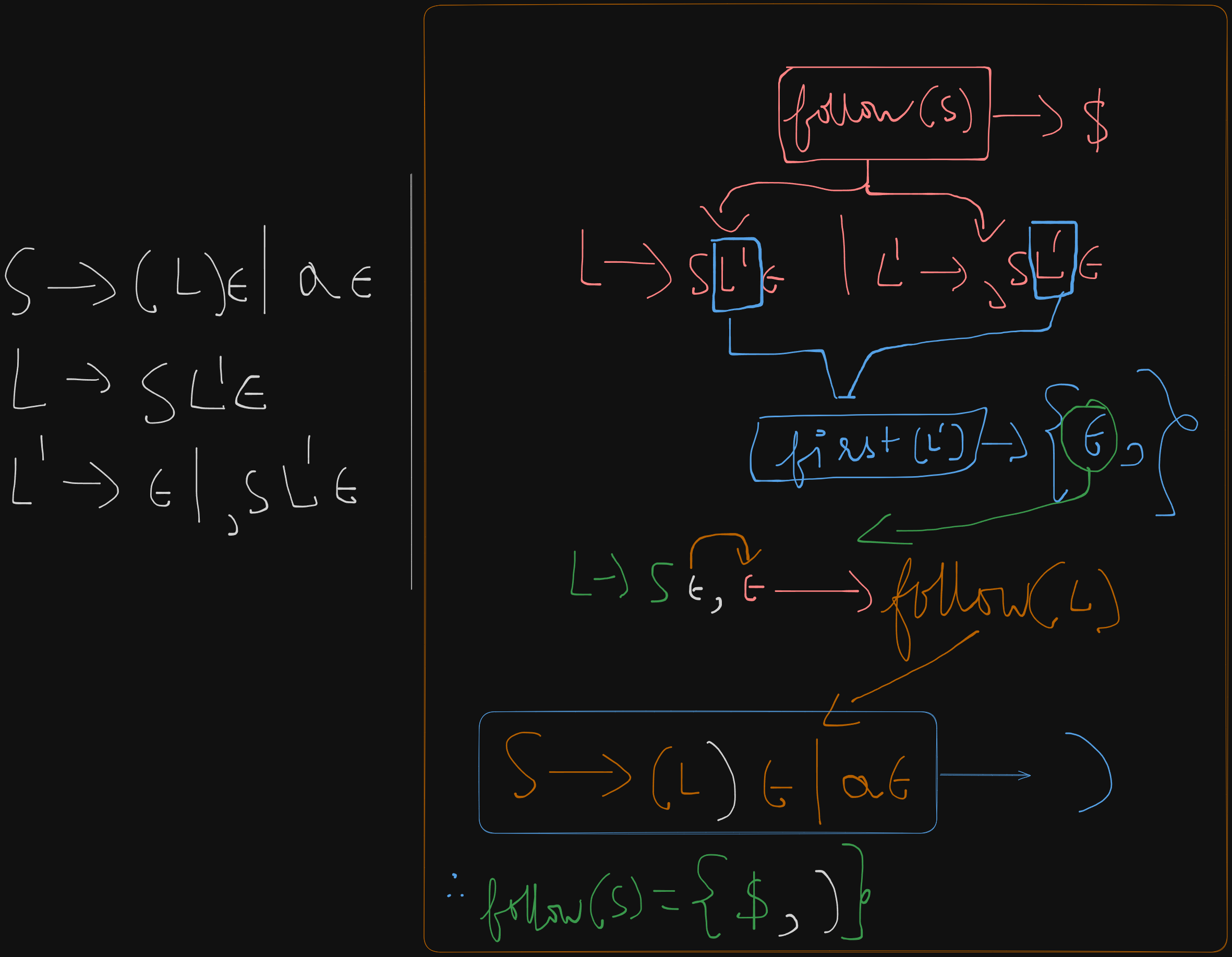
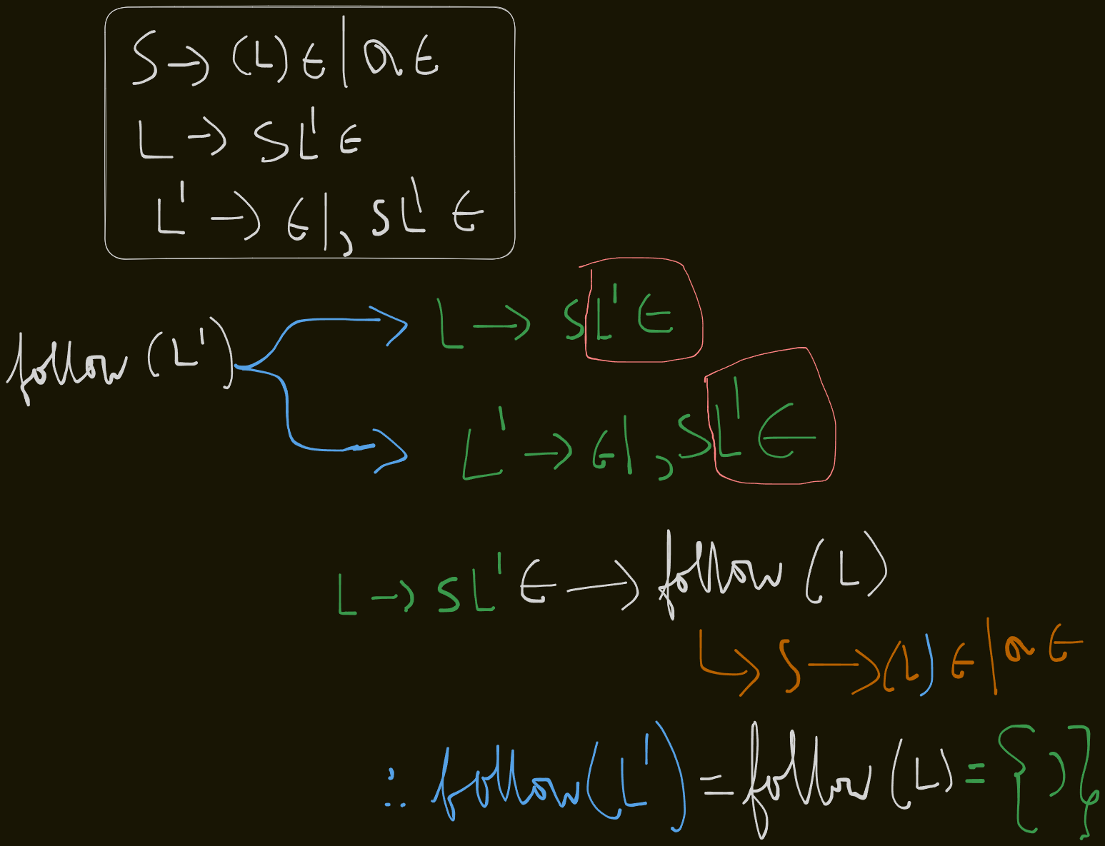
follow(S) = {$, first(L')} = {$, )}
follow(L) = {)}
`follow(L’) = follow(L) = )
Now we assign numbers to the productions :
S -> (L) = 1
S -> a = 2
L -> SL' = 3
L' -> ε = 4
L' -> ,SL' = 5
Now we create the parse table with each column header containing a terminal symbol .
$ is always present as an extra terminal in the table
We CANNOT use ε as a column header in the parse table.
We need to fill the empty part of the table with the numbered productions
| Variables | ( | ) | a | , | $ |
|---|---|---|---|---|---|
| S | |||||
| L | |||||
| L’ |
So we take production 1
S -> (L) and we find the first() of it’s RHS, which is just (
So we fill 1 under the ( symbol.
| Variables | ( | ) | a | , | $ |
|---|---|---|---|---|---|
| S | 1 | ||||
| L | |||||
| L’ |
As for production 2, S -> a, we just write 2 under a symbol in the table.
| Variables | ( | ) | a | , | $ |
|---|---|---|---|---|---|
| S | 1 | 2 | |||
| L | |||||
| L’ |
For production 3 L -> SL', first(L) = S, so we find first of S which is {(, a}
So we write 3 under the ( symbol and the a symbol
| Variables | ( | ) | a | , | $ |
|---|---|---|---|---|---|
| S | 1 | 2 | |||
| L | 3 | 3 | |||
| L’ |
For production 4, L' -> ε , we see that we have ε on the RHS. So we find the follow(L') which is {)}
So we write 4 under the ) symbol.
| Variables | ( | ) | a | , | $ |
|---|---|---|---|---|---|
| S | 1 | 2 | |||
| L | 3 | 3 | |||
| L’ | 4 |
And lastly for production 5, L' -> ,SL', the first(L') = {,}
So we write 5 under the , symbol.
| Variables | ( | ) | a | , | $ |
|---|---|---|---|---|---|
| S | 1 | 2 | |||
| L | 3 | 3 | |||
| L’ | 4 | 5 |
Now if any cell within the LL(1) parse table has more than one entry in it, then the given grammar is NOT LL(1) compatible.
Here we see that the populated cells have only one entry each.
So, the given grammar,
S -> (L) | a
L -> SL'
L' -> ε | ,SL'
is LL(1) compatible.
Example 2
S -> aSbS | bSaS | εSo we can re-write this grammar as :
S -> aSbSε | bSaSε | εWe need to check whether this grammar is LL(1) compatible or not.
First sets
first(S) = abε
Follow sets
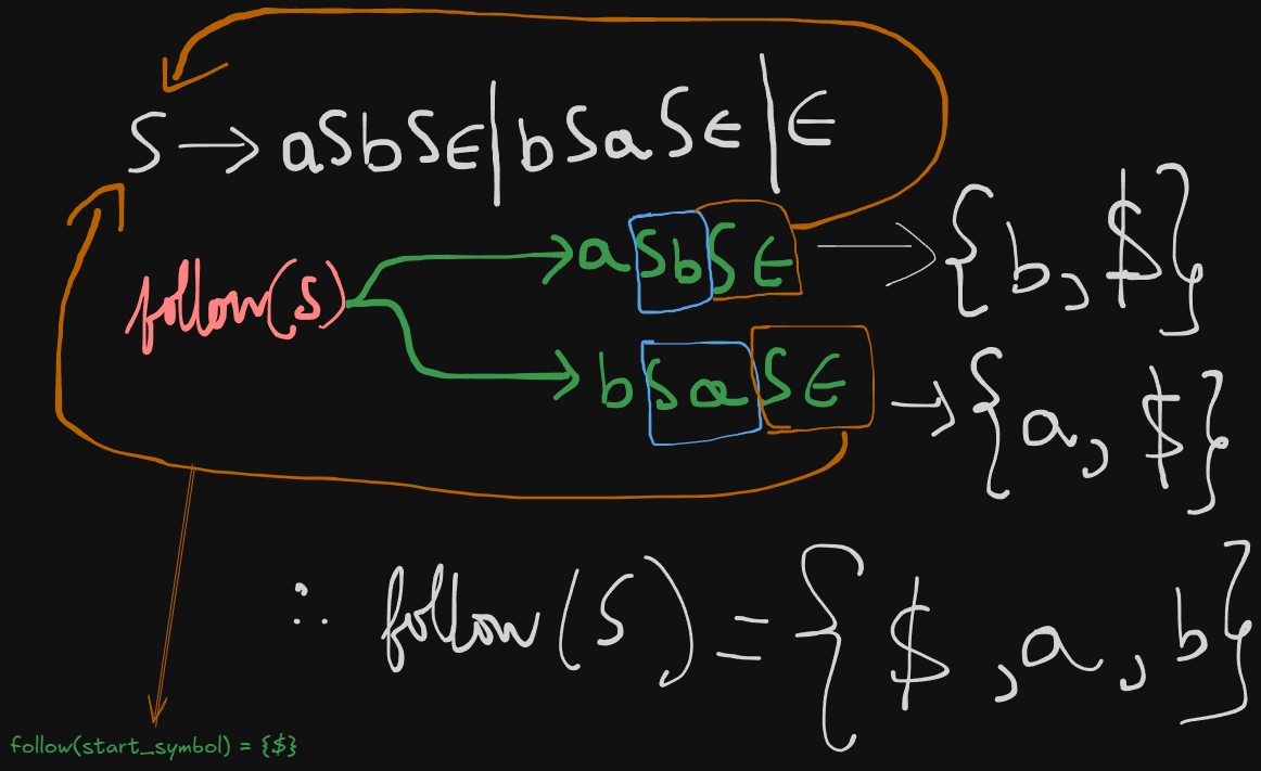
follow(S) = {$, a, b}
Therefore the LL(1) parsing table will be:
| Variables | a | b | $ |
|---|---|---|---|
| S |
Now we number the productions :
S -> aSbS = 1.
S -> bSaS = 2.
S -> ε = 3.
Starting with production 1, we find the first(S) which is a.
So we write 1 under the column of a symbol.
| Variables | a | b | $ |
|---|---|---|---|
| S | 1 |
For production 2, first(S) = b.
So we write 2 under the b symbol.
| Variables | a | b | $ |
|---|---|---|---|
| S | 1 | 2 |
For production 3, we see that first(S) = ε. So it will result in a follow(S) which is {$, a, b}.
So we will write 3 in all the cells of the table.
Existing values will assume a fractional form as follows:
| Variables | a | b | $ |
|---|---|---|---|
| S | 1/3 | 2/3 | 3 |
So here we see that two cells contain more than one value.
So the grammar :
S -> aSbS | bSaS | εis NOT, LL(1) compatible.
Checking if a grammar is SLR(1) compatible.
SLR(1) parsing belongs to the parsing type of Bottom-up parsing where the entire production is scanned first by the parser to the bottom then reduced back to it’s start symbol at the top.
Let’s say we have been given an example grammar:
E -> T + E | T
T -> id- We number the productions as we did previously.
E -> T + E = 1.
E -> T = 2.
T -> id = 3.
- We then, augment the grammar by adding a new production rule which points to the start symbol.
E' -> E
So the new augmented grammar becomes:
E' -> E
E -> T + E
E -> T
T -> id- Build the LR(0) canonical item sets.
- Build the LR(0) Action and Go-To tables
- Build the SLR(1) Action Table from the LR(0) Action Table
- If there are no conflicts (shift-reduce or reduce-reduce), then the grammar is SLR(1) compatible
Recapping the concepts of LR(0) canonical items, shifting and reduction LR(0) parsing.
The parsing process happens with the help of certain items called canonical items. In this instance, these are called LR(0) canonical items as SLR(1) parsing depends on LR(0) canonical items.
So here the parser (atleast in theory let’s assume we have a machine called a parser), will scan through all the symbols one at a time.
We visually represent this process by using a dot .
So, there will be a stage when the dot is before a variable (meaning it’s not scanned), and a stage after the variable, where it’s scanned( which means that production is ready to be reduced.)
So we get these :
-
Production:
E' -> E- Items:
E' -> .E   // Initial item for the start symbol
E' -> E. // The dot is after the entire production, meaning it's ready for reduction-
Production:
E -> T + E- Items:
E -> .T + E   // Before anything is parsed
E -> T . + E  // After parsing `T`
E -> T + .E   // After parsing `T +`
E -> T + E. // After parsing `T + E`- Production:
E -> T- Items:
E -> .T      // Before `T` is parsed
E -> T. // After `T` is parsed (ready for reduction)- Production:
T -> id- Items:
T -> .id     // Before `id` is parsed
T -> id.     // After `id` is parsed (ready for reduction)
So, the LR(0) items (without closure) are:
E' -> .E
E' -> E.
E -> .T + E
E -> T . + E
E -> T + .E
E -> T + E.
E -> .T
E -> T.
T -> .id
T -> id.
Now these items are called LR(0) canonical items without closure.
What is closure by the way?
It’s basically the expansion of non-terminal variables, revealing all possible productions like a traversal, and adding unexplored non-terminals to the right of the dot, to consider them as parsed.
Like opening a folder to see their contents inside.
It only works on non-terminal variables.
So after applying closure, the items will be grouped into sets, called canonical item sets.
So here we have the first production:
E' -> .E
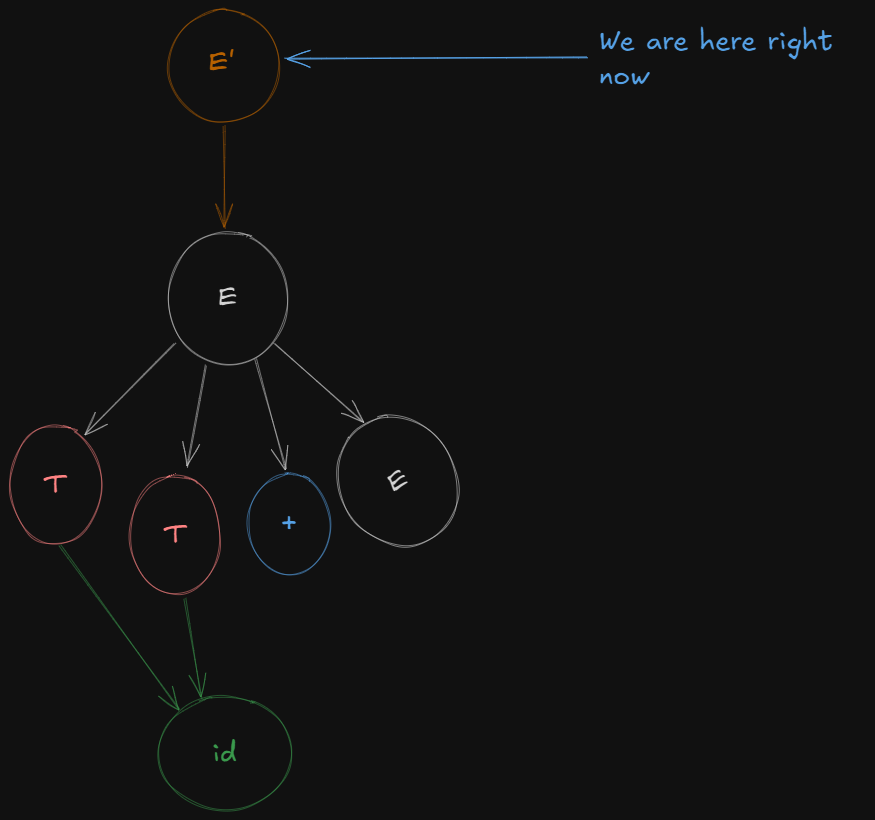
So here to form a closure of E', it needs to be expanded.

So accommodating all expansions of E', we get the first LR(0) canonical item set as :
E' → .E
E → .T + E
E → .T
T → .id
Now to open the folder of E or expand on E, the parser needs to shift over E first so that it’s ready for reduction.
So we get a new LR(0) canonical item set as :
E' -> E.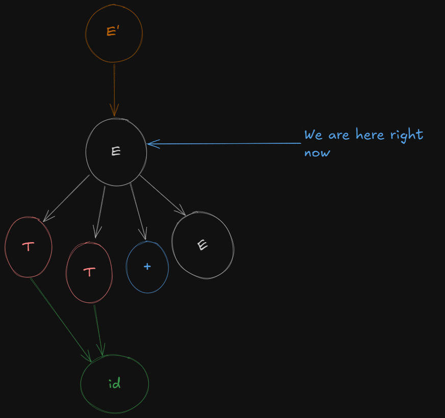
Next we open the folder of E or expand on E (however you say it).

So we get to see the two productions which E leads to and the parser shifts over the first variable, T in both cases, meaning the variable T is ready for reduction.
So we get a new LR(0) canonical item set as:
E → T. + E
E → T.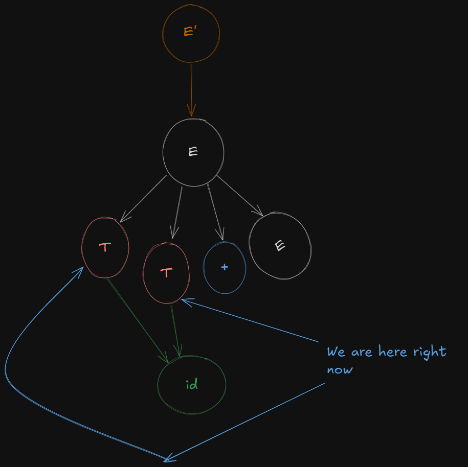
Now we can’t parse the next variable as it’s a terminal variable and closure only works on non-terminal variables, but the parser can still shift beyond the terminal to access any remaining non-terminals.
So the parser just shifts over the terminal symbol + to get a new production
E -> T + .E
So, we get a new canonical item set as :
E -> T +. E
E → .T + E
E → .T
T → .id
Why are not the remaining productions shifted over too?
E → .T + E
E → .T
T → .id
These?
Because :
-
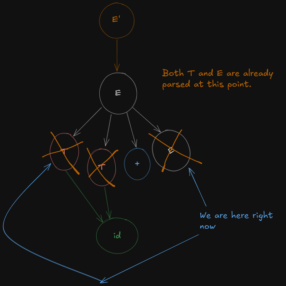
Thas already been parsed over, so we don’t need to shift the dots again over the remainingT.In:
E → T. + E E → T.Thas already been shifted over.So we don’t expand T again.
And in :
E' -> E.Ehas already been parsed completely.So even after shifting over to get :
E → T + E.We don’t expand E again.
-
The way the shifting is done is dictated by the rules of the original grammar. These “canonical item sets” we see are in-between phases of parsing, so we don’t follow their “rules” to shift over again.
So from , after shifting the dot over E we get a new LR(0) canonical item as :
E → T + E.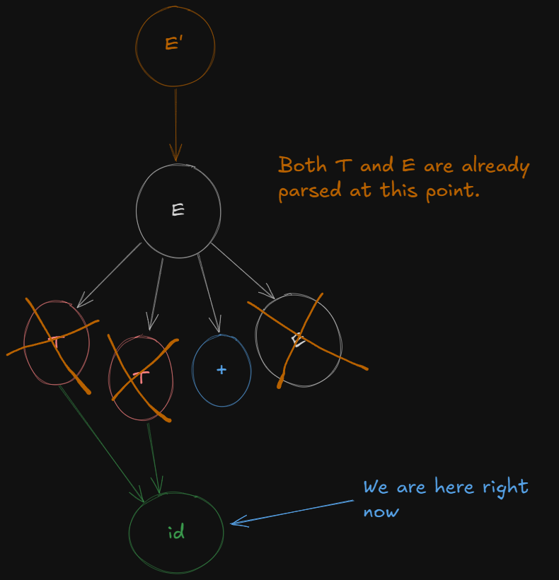
And shifting the dot over terminal id we get the last LR(0) canonical item set as :
T -> id.And thus finally all non-terminals have been expanded and are ready for reduction.
What Exactly is Reduction in LR Parsing?
Reduction in LR parsing means that the parser has matched a sequence of input symbols that corresponds to the right-hand side (RHS) of a production rule, and it now replaces this sequence with the left-hand side (LHS) of the production.
Reduction is the reverse of derivation:
- In derivation, you expand non-terminals into terminals using production rules.
- In reduction, you collapse terminals back into non-terminals using the production rules.
It’s like a substitution method, but only works if it’s possible to substitute the entire input/production rule back to the original numbered production.
Reduction only works, if the entire production rule / terminal has been parsed, and end of input has been reached. The parser then checks whether it’s possible to reduce the entire rule / terminal, back to the augmented start symbol.
This is how reduction works in bottom-up parsing, where it gradually builds back up to the start symbol.
What exactly is Shifting in LR parsing?
Shifts (S):
- Shift means to “read” a symbol from the input and move to a new state.
S3means Shift the input symbol (i.e., read it) and then move to state3.
The number after S refers to the state the parser should transition to after the shift. Here’s how it works:
- The current state looks at the next input symbol (let’s say it’s
+). - If the table entry says
S3, it means “Shift the input symbol+, consume it, and go to state3”.
For example, if you’re in state 0 and the next input symbol is id, the Action table might say S5. This means the parser will shift (consume id) and move to state 5.
Creating the LR(0) Action and Go-To Tables
Recapping our LR(0) canonical items
- I₀:
E' → .E
E → .T + E
E → .T
T → .id- I₁:
E' -> E.- I₂:
E -> T. + E
E -> T.- I₃:
E → T + .E
E → .T + E
E → .T
T → .id- I₄: from (I3),
E -> T + .E
E -> T + E.- I5: (from I0)
T -> id.And our numbered productions
We number these productions as 1, 2 and 3
E -> T + E = 1
E -> T = 2
T -> id = 3
Creating the LR(0) Action Table.
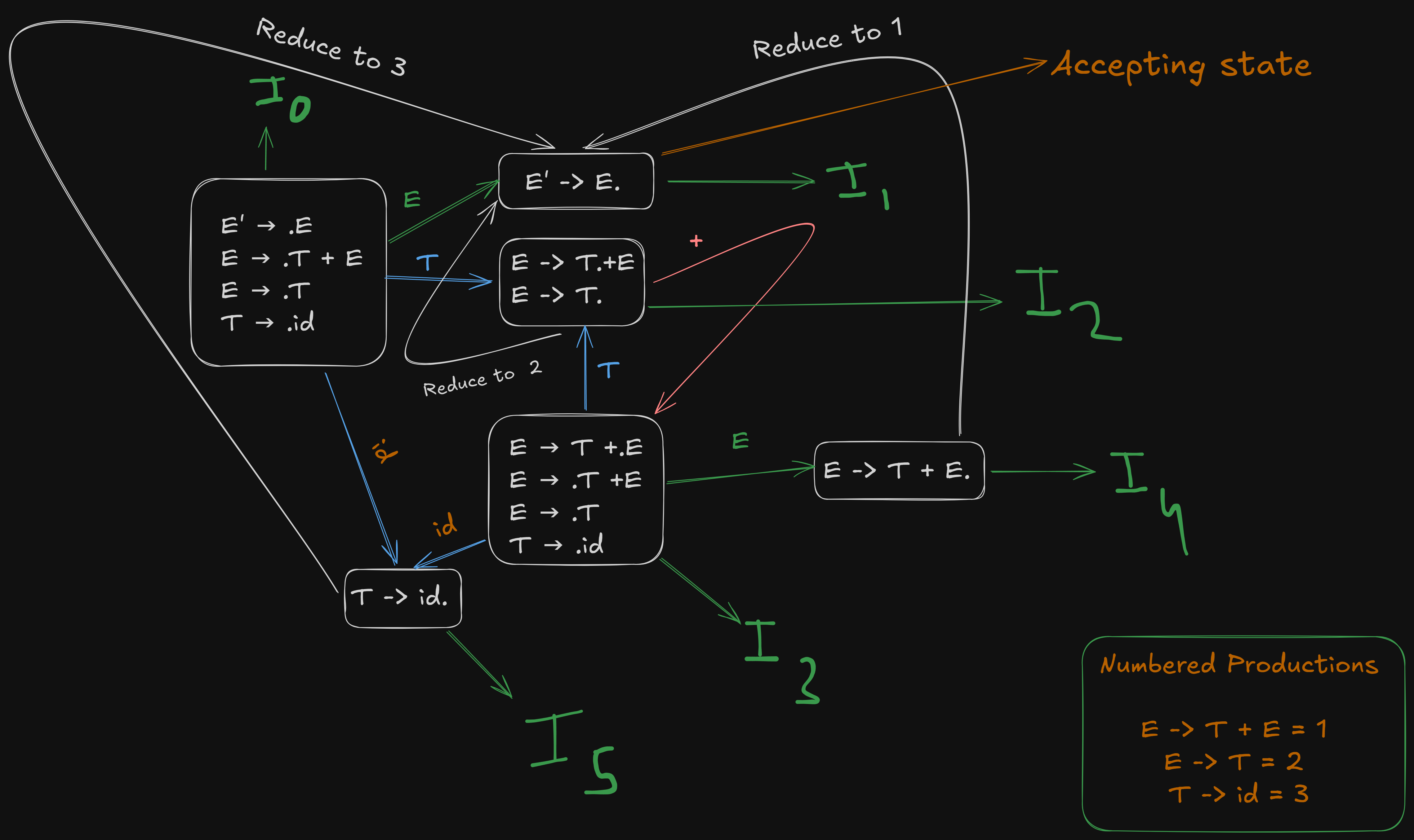
All the state transitions are depicted in this picture.
The action table denotes transitions over terminal symbols and the reductions
We create the action table as follows :
The column headers are all the terminal symbols because that’s where the shifting takes place.
| States | id | + | $ |
|---|---|---|---|
| | |||
| | |||
| | |||
| | |||
| | |||
| |
For terminal id we see that goes to from the image.
So will shift over id to
So we write S5 to represent “Shift to State 5”.
| States | id | + | $ |
|---|---|---|---|
| | S5 | ||
| | |||
| | |||
| | |||
| | |||
| |
The augmented grammar has E' as the new start symbol, and the goal of the parser is to reduce everything down to E' → E.
In we see that E' -> E., the input has been reduced to the start symbol E', and the dot at the end means that the entire derivation of the grammar has been successfully parsed.
So is the accept state.
| States | id | + | $ |
|---|---|---|---|
| | S5 | ||
| | accept | ||
| | |||
| | |||
| | |||
| |
The reason the accept word is written under $ symbol is because there is no shift/reduction happening here.
For we see that it shifts over to for + terminal.
So we write S3 denoting “Shift to State 3”
The parser sees that E -> T. is present in which can be completely reduced back to numbered production 2.
So we write R2, to represent Reduction to rule 2, in all the columns of that row.
| States | id | + | $ |
|---|---|---|---|
| | S5 | ||
| | accept | ||
| | R2 | S3/R2 | R2 |
| | |||
| | |||
| |
Now dealing with , we see that it shifts over id to .
So we write S5 to represent “Shift to State 5”.
| States | id | + | $ |
|---|---|---|---|
| | S5 | ||
| | accept | ||
| | R2 | S3/R2 | R2 |
| | S5 | ||
| | |||
| |
Now for , E -> T + E. can be completely reduced back to production 1. So we write R1 in the entire row, denoting Reduce to rule 1.
| States | id | + | $ |
|---|---|---|---|
| | S5 | ||
| | accept | ||
| | R2 | S3/R2 | R2 |
| | S5 | ||
| | R1 | R1 | R1 |
| |
And for , T -> id., can be completely reduced back to production 3. So we write R3 in the entire row, denoting Reduce to rule 3.
| States | id | + | $ |
|---|---|---|---|
| | S5 | ||
| | accept | ||
| | R2 | S3/R2 | R2 |
| | S5 | ||
| | R1 | R1 | R1 |
| | R3 | R3 | R3 |
This is the LR(0) Action Table, which is necessary to understand before creating the SLR(0) Action Table.
Creating the LR(0) Go-To table
Referencing the image again :

The Go-To table denotes shifts over all non-terminal variables.
The non-terminal shifts here are only for
to for E ⇒ S1
to for T ⇒ S2
to for E ⇒ S4
to for T ⇒ S2
So this is our initial Go-To table.
| State | E | T |
|---|---|---|
| | ||
| | ||
| | ||
| | ||
| |
And after filling in all the transitions, we get :
| State | E | T |
|---|---|---|
| | S1 | S2 |
| | ||
| | S4 | S2 |
| | ||
| |
Here is our final LR(0) Go-to Table.
The actual LR(0) parsing table is the combination of both of these tables.
| States | id | + | $ | E | T |
|---|---|---|---|---|---|
| I0 | S5 | I1 | I2 | ||
| I1 | accept | ||||
| I2 | R2 | S3/R2 | R2 | ||
| I3 | S5 | I4 | I2 | ||
| I4 | R1 | R1 | R1 | ||
| I5 | R3 | R3 | R3 |
Creating the SLR(1) parsing table.
The SLR(1) Go-To table is the same as the LR(0) Go-To table, however there is a significant difference between the Action Tables of the two.
As we can see in the LR(0) parsing table, one cell has both a shift and a reduction at the same time.
This is called a shift-reduce conflict, which SLR(1) and LR(0) DO NOT allow.
So to make the action table for SLR(1) we need to see if the removal of the shift-reduce conflict and the reduce-reduce conflict is possible or not. If yes, then the given grammar will be compatible with an SLR(1) parser.
So, we start with the current LR(0) Action Table
| States | id | + | $ |
|---|---|---|---|
| | S5 | ||
| | accept | ||
| | R2 | S3/R2 | R2 |
| | S5 | ||
| | R1 | R1 | R1 |
| | R3 | R3 | R3 |
has a reduction to rule 2, and a shift reduce conflict as well.
So we need to find the follow of the LHS of this rule here.

So we write R2 under $$$ symbol
| States | id | + | $ |
|---|---|---|---|
| | S5 | ||
| | accept | ||
| | S3 | R2 | |
| | S5 | ||
| | R1 | R1 | R1 |
| | R3 | R3 | R3 |
For :

So we write R1 under $$$ symbol
| States | id | + | $ |
|---|---|---|---|
| | S5 | ||
| | accept | ||
| | S3 | R2 | |
| | S5 | ||
| | R1 | ||
| | R3 | R3 | R3 |
And for :

Therefore we will place R3 under both + and $$$ symbols
| States | id | + | $ |
|---|---|---|---|
| | S5 | ||
| | accept | ||
| | S3 | R2 | |
| | S5 | ||
| | R1 | ||
| | R3 | R3 |
Now we see that there are no-more shift-reduce conflicts, so this grammar is SLR(1) compatible, but LR(0) incompatible.
This means that SLR(1) may accept extra grammars which are not LR(0) compatible.
Checking whether a grammar is LALR(1) compatible or not
LALR(1) parser is another type of Top-Down parser which is based on LR(1) parser.
The LR(1) parser works on LR(1) grammar which is slightly different than it’s LR(0) counterpart.
The process to generate the LR(1) canonical items is similar to the LR(0) process, except that we need to track a lookahead symbol.
- Construct LR(1) canonical items
- Construct LR(1) Action and Go-To table
- See if merging of states is possible or not, without any conflicts.
- If possible, then the grammar is LALR(1) compatible, else it is not LALR(1) compatible.
So let’s say we have an example grammar here:
S -> aAd | bBd | aBe | bAe
A -> c
B -> c
We proceed similarly, first augmenting the grammar and numbering the original productions.
S' -> S
S -> aAd | bBd | aBe | bAe
A -> c
B -> c
S->aAd = 1
S-> bBd = 2
S -> aBe = 3
S -> bAe = 4
A -> c = 5
B -> c = 6
Step 2. Construct the first unclosured LR(1) item
:
S' -> .S    , [$]
S  -> .aAd  , [$]
S  -> .bBd  , [$]
S  -> .aBe  , [$]
S  -> .bAe  , [$]
A -> .c, [$]
B -> .c, [$]
where the dot indicates that it hasn’t parsed anything yet, and each production of S is followed by the lookahead symbol $.
We get a new canonical item as
S' -> S. , [$]which is the accepting state as the original start symbol has been parsed.
Step 3. Construct Go-To operations on terminal symbols first.
For a ,
We can get a new canonical item
S  -> a.Ad  , [$]
S  -> a.Be  , [$]
Now we see that the dot is in front of non-terminals A and B, so they need to expanded further.
A -> .c, [$]
B -> .c, [$]
However in this instance the lookahead for c won’t be $, since there are terminals d and e after the expansion of the non-terminals A and B. So we the new lookahead symbols will be d and e respectively
A -> .c, [d]
B -> .c, [e]
So the final becomes :
S  -> a.Ad  , [$]
S  -> a.Be  , [$]
A -> .c, [d]
B -> .c, [e]
In a similar way, we can find the next canonical item for terminal b.
S  -> b.Bd  , [$]
S  -> b.Ae  , [$]
A -> .c, [e]
B -> .c, [d]
Step 4. Perform Go-To operations on non-terminals.
Right now, the parser is at a stage where it needs to shift and parse over the non-terminal symbols before parsing the remaining terminal symbols.
So from items and , we get:
:
S -> aA.d , [$]:
S -> aB.e , [$]:
S -> bA.e, [$]:
S -> bB.d, [$]Step 5. Perform Go-To operations on remaining terminal symbols
Now that the non-terminal symbols have been parsed, we can parse the remaining terminal symbols
There are still a few remaining terminals, c, d and e.
For d and e
And from states , and , we get:
S -> aAd. ,[$] →
S -> aBe. , [$] →
And from states and , we get:
S -> bBd. , [$] →
S -> bAe. , [$] →
And for c:
We see that from : A -> .c, [d] and B -> .c, [e] can have the dot shifted over to get
:
A -> c. , [d]
B ->c. , [e]
And from : A -> .c, [e] and B -> .c, [d] can have the dot shifted over to get
:
A -> c. , [e]
B ->c. , [d]
So, the final recollection of all LR(1) canonical items

Step 6. Building the LR(1) and Go-To tables
The Action table deals with shifts, reduces, and accepts. We look at the items with:
- Shift actions: When there is a dot before a terminal symbol.
- Reduce actions: When a production is completed (dot at the end of a rule).
- Accept action: When we have
S' -> S. , [$]in some item set.
We construct our empty LR(1) action table
| States | a | b | c | d | e | $ |
|---|---|---|---|---|---|---|
Referencing our image again,
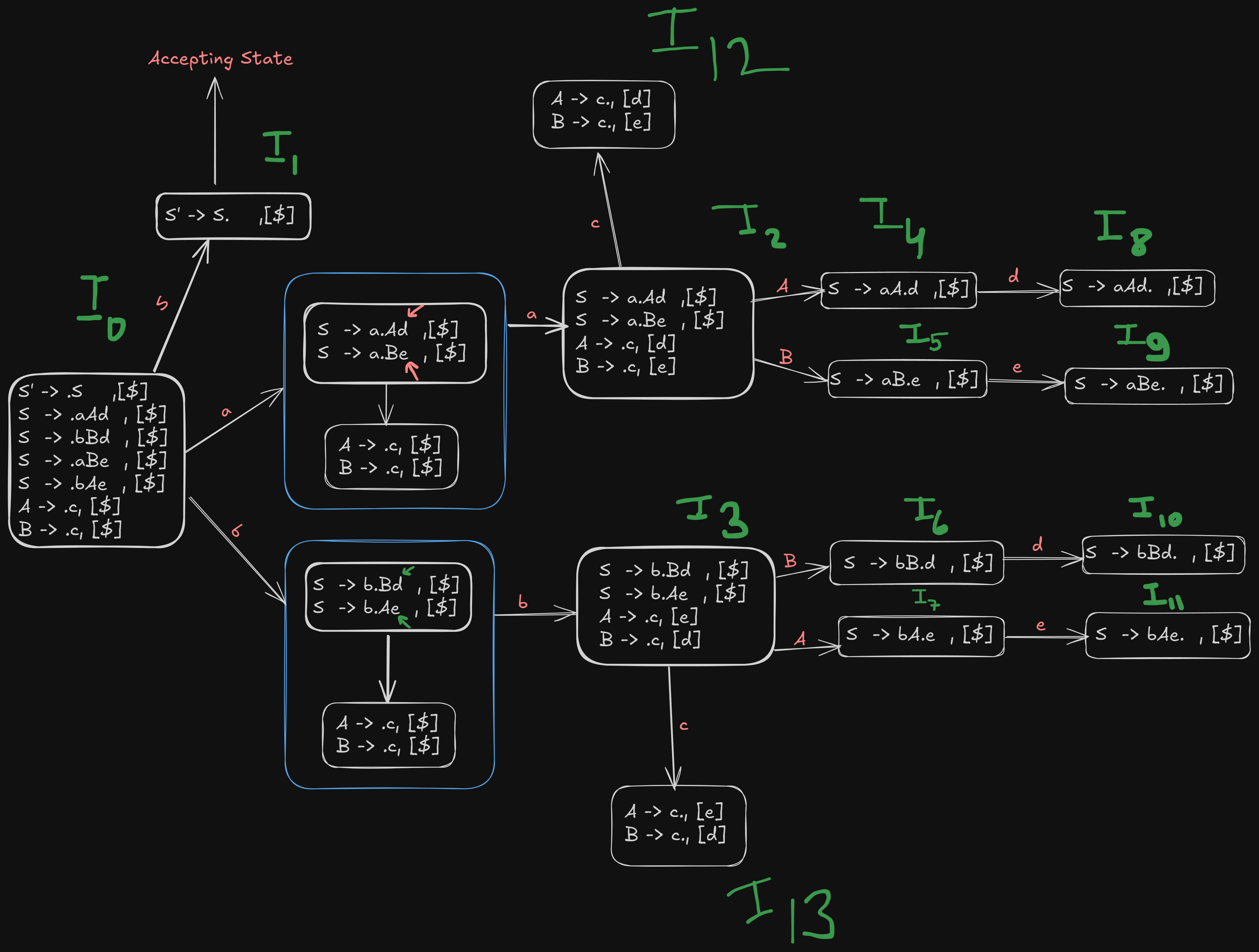
We see that for terminal a, goes to state
For terminal b, goes to state
And is the accepting state here.
Therefore we denote those shifts with S2 and S3
| States | a | b | c | d | e | $ |
|---|---|---|---|---|---|---|
S2 | S3 | |||||
| accept | ||||||
For terminal c, goes to and goes to
So, we denote those shifts using S12 and S13
| States | a | b | c | d | e | $ |
|---|---|---|---|---|---|---|
S2 | S3 | |||||
| accept | ||||||
S12 | ||||||
S13 | ||||||
For terminal d, and go to and each.
So we denote the shifts using S8 and S10.
| States | a | b | c | d | e | $ |
|---|---|---|---|---|---|---|
S2 | S3 | |||||
| accept | ||||||
S12 | ||||||
S13 | ||||||
S8 | ||||||
S10 | ||||||
For terminal e, and go to and each.
So we denote those shifts using S10 and S11.
| States | a | b | c | d | e | $ |
|---|---|---|---|---|---|---|
S2 | S3 | |||||
| accept | ||||||
S12 | ||||||
S13 | ||||||
S8 | ||||||
S9 | ||||||
S10 | ||||||
S11 | ||||||

Now from the image, we see that, states to are all reducible states.
Recapping our original numbered productions:
S->aAd = 1
S-> bBd = 2
S -> aBe = 3
S -> bAe = 4
A -> c = 5
B -> c = 6
So the reduction goes like this,
has S -> aAd. ,[$] which can be reduced back to rule 1
has S -> aBe. , [$], which can be reduced back to rule 3
has S -> bBd. , [$], which can be reduced back to rule 2
has S -> bAe. , [$], which can be reduced back to rule 4
has :
A -> c., [d]
B -> c., [e]
which reduce to rules 5 and 6
and has:
A -> c., [e]
B -> c., [d]
which, again reduce to rule 5 and 6.
So the resulting Action Table accordingly will be:
| States | a | b | c | d | e | $ |
|---|---|---|---|---|---|---|
S2 | S3 | |||||
| accept | ||||||
S12 | ||||||
S13 | ||||||
S8 | ||||||
S9 | ||||||
S10 | ||||||
S11 | ||||||
R1 | ||||||
R3 | ||||||
R2 | ||||||
R4 | ||||||
R5 | R6 | |||||
R6 | R5 |
Constructing the LR(1) Go-To table
As usual, the Go-To table will focus on transitions over non-terminal symbols
We have non-terminals A and B.

Referencing our image again, we see that :
goes to for non-terminal S.
goes to for non-terminal A.
goes to for non-terminal B.
goes to for non-terminal B.
goes to for non-terminal A.
So the final LR(1) parsing table will be :
| States | a | b | c | d | e | $ | S | A | B |
|---|---|---|---|---|---|---|---|---|---|
S2 | S3 | S1 | |||||||
| accept | |||||||||
S12 | S4 | S5 | |||||||
S13 | S7 | S6 | |||||||
S8 | |||||||||
S9 | |||||||||
S10 | |||||||||
S11 | |||||||||
R1 | |||||||||
R3 | |||||||||
R2 | |||||||||
R4 | |||||||||
R5 | R6 | ||||||||
R6 | R5 |
Step 7. Checking if merging of states is possible or not.
LALR parser works by merging similar states into a single state, thus reducing the number of shifts.
Here we see that we have two similar states under different lookaheads d and e
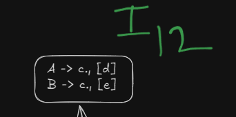
and
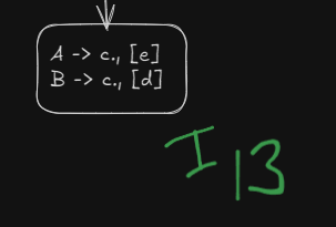
Both can be merged into a single state, however this will lead to a reduce-reduce conflict which LALR(1) parser DOES NOT allow.
How does the reduce-reduce conflict arise?
Well, since these two states had initially separate reductions under the different lookaheads
R5 | R6 | ||||
|---|---|---|---|---|---|
R6 | R5 |
On being merged :
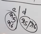
The reductions will be in a single cell now, which will cause a reduce-reduce conflict.
Thus this grammar is NOT LALR(1) compatible.
However, for an example grammar which is indeed compatible, check example 2 from this video :
https://www.youtube.com/watch?v=GOlsYofJjyQ&list=PLxCzCOWd7aiEKtKSIHYusizkESC42diyc&index=15
Operator Precedence Parsing
https://www.youtube.com/watch?v=7K2U4Otqhpk
Well, operator precedence parsing, works differently than the other parsers. It works a specific type of grammar called “Operator precedence grammar”, which should not have :
- Epsilon (ε) productions.
- Two consecutive non-terminals on the right-hand side of any production.
Define Operator Precedence Rules
We establish precedence between the terminal operators based on their natural precedence and associativity rules:
- Multiplication (
*) has higher precedence than addition (+). - Parentheses (
(and)) have the highest precedence, and()must be treated as grouping. - Identifiers (
id) represent operands.
| Operator | Associativity | Precedence |
|---|---|---|
id | Higher than operators precedence | 1 |
( ) | Highest precedence | 2 |
* | Left-to-right | 3 |
+ | Left-to-right | 4 |
$ | Lowest precedence among all | 5 |
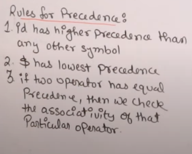
In this table:
- Parentheses have the highest precedence and override all other operators.
- Multiplication (
*) has a higher precedence than addition (+), so multiplication is performed before addition. - Both
*and+are left-associative, meaning expressions are evaluated from left to right when these operators appear in sequence. - Identifiers (operands) have precedence lower than operators.
- The
$symbol has the lowest precedence.
Creating the Operator Precedence parsing table.
So let’s say we have this grammar :

This is our empty operator precedence parsing table.
| Terminals | + | * | id | $ |
|---|---|---|---|---|
+ | ||||
* | ||||
id | ||||
$ | ||||
We fill in values with either > or <.
And we remember these rules.
Since the operators are left-associative, this means that the in any sequence of operators, the leftmost one is parsed first. This means that in the case of the same operators, the leftmost one will get the higher priority. And in case of different operators, the precedence will give them value.
In case of operands next to each other, their relations are not parsed.
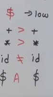
However operand-operator relations are parsed and the operand is parsed before the operator is parsed.
$ is always parsed last no matter what the order.
$ - $ marks the accept state.
Following this logic, from these rules, we set up the operators precedence parsing table.
Initially we see that we have the + operator against the + operator. Since it is left associative, the + operator will get the higher priority, and we will put > next to it.
| Terminals | + | * | id | $ |
|---|---|---|---|---|
+ | > | |||
* | ||||
id | ||||
$ |
Next up, the * operator is up against the + operator. Since * operator has a higher priority, we will put > next to it.
| Terminals | + | * | id | $ |
|---|---|---|---|---|
+ | > | < | < | > |
* | ||||
id | ||||
$ |
Next up we had id, which is an operand. Operands has lower priority than operators, so we will put a < next to it.
And then we have the $ symbol, which has the lowest priority. So we will put a < next to it.
| Terminals | + | * | id | $ |
|---|---|---|---|---|
+ | > | < | < | > |
* | ||||
id | ||||
$ |
For the next column, we will follow the rules as before and get this column :
| Terminals | + | * | id | $ |
|---|---|---|---|---|
+ | > | < | < | > |
* | > | > | < | > |
id | ||||
$ |
For the operand id, we will follow the same rules as before.
| Terminals | + | * | id | $ |
|---|---|---|---|---|
+ | > | < | < | > |
* | > | > | < | > |
id | > | > | ||
$ |
However as we have seen before : operand-operand rules are not parsed. So we leave the field blank for id against id.
| Terminals | + | * | id | $ |
|---|---|---|---|---|
+ | > | < | < | > |
* | > | > | < | > |
id | > | > | __ | > |
$ |
And lastly $ has the lowest precedence so we put a < in it’s field.
| Terminals | + | * | id | $ |
|---|---|---|---|---|
+ | > | < | < | > |
* | > | > | < | > |
id | > | > | __ | > |
$ |
And for the column of $ we follow the same rules as before to get :
| Terminals | + | * | id | $ |
|---|---|---|---|---|
+ | > | < | < | > |
* | > | > | < | > |
id | > | > | __ | > |
$ | < | < | < | accept |
And when $ is against $, it is the accepting state.
Parsing a string from the Operator-Precedence Parsing Table
Here are our numbered productions from the grammar
T -> T + T = 1
T -> T * T = 2
T -> id = 3
Now, let’s parse a string from this table : id + id * id.
For this, we make this table, much more convenient than having separate stack and input buffer tables.
And we start with the $ symbol in the stack and the given string in the input section along with $ at it’s end
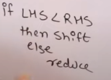
We follow the main rule here :
| Stack | Relation | Input | Comment |
|---|---|---|---|
$ | id + id * id $ | ||
We parse the string by comparing the current symbol in the stack with the current character in the string (reading from left to right).
So right now we have $ in the stack which needs to be compared to id.
Looking at our parse table, we see that $ < id so we shift over id to the the stack and remove the current character from the input buffer. We write shift id in the comment section
General rule :
If Stack < input, we shift the current symbol in the input.. If Stack > input, we reduce the top of the stack..
| Stack | Relation | Input | Comment |
|---|---|---|---|
$ | < | id + id * id $ | Shift id |
$ id | + id * id $ |
Now we compare id from the stack to + from the input.
We see that id > +, so we reduce id to our numbered production 3
In this case, we replace id by the reduced production’s start symbol.
No change takes place to the input buffer during reduction.
| Stack | Relation | Input | Comment |
|---|---|---|---|
$ | < | id + id * id $ | Shift id |
$ id | > | + id * id $ | Reduce id to 3 |
$ T | + id * id $ |
We don’t compare non-terminals to terminals, so we compare the terminal before T , $ to +
We see that $ < +, so we shift +.
| Stack | Relation | Input | Comment |
|---|---|---|---|
$ | < | id + id * id $ | Shift id |
$ id | > | + id * id $ | Reduce id to 3 |
$ T | < | + id * id $ | Shift + |
$ T + | id * id $ |
We now compare + to id.
We see that + < id, so we shift id
| Stack | Relation | Input | Comment |
|---|---|---|---|
$ | < | id + id * id $ | Shift id |
$ id | > | + id * id $ | Reduce id to 3 |
$ T | < | + id * id $ | Shift + |
$ T + | < | id * id $ | Shift id |
$ T + id | * id $ |
We now compare id to *.
We see that id > *, so we reduce id to production 3.
| Stack | Relation | Input | Comment |
|---|---|---|---|
$ | < | id + id * id $ | Shift id |
$ id | > | + id * id $ | Reduce id to 3 |
$ T | < | + id * id $ | Shift + |
$ T + | < | id * id $ | Shift id |
$ T + id | > | * id $ | Reduce id to 3 |
$ T + T | * id $ |
We now compare + to *.
We see that + < *, so we shift *.
| Stack | Relation | Input | Comment |
|---|---|---|---|
$ | < | id + id * id $ | Shift id |
$ id | > | + id * id $ | Reduce id to 3 |
$ T | < | + id * id $ | Shift + |
$ T + | < | id * id $ | Shift id |
$ T + id | > | * id $ | Reduce id to 3 |
$ T + T | < | * id $ | Shift * |
$ T + T * | id $ |
We now compare * to id.
We see that * < id, so we shift id.
| Stack | Relation | Input | Comment |
|---|---|---|---|
$ | < | id + id * id $ | Shift id |
$ id | > | + id * id $ | Reduce id to 3 |
$ T | < | + id * id $ | Shift + |
$ T + | < | id * id $ | Shift id |
$ T + id | > | * id $ | Reduce id to 3 |
$ T + T | < | * id $ | Shift * |
$ T + T * | < | id $ | Shift id |
$ T + T * id | $ |
We now compare id to $.
We see that id > $, so we reduce id to production 3.
| Stack | Relation | Input | Comment |
|---|---|---|---|
$ | < | id + id * id $ | Shift id |
$ id | > | + id * id $ | Reduce id to 3 |
$ T | < | + id * id $ | Shift + |
$ T + | < | id * id $ | Shift id |
$ T + id | > | * id $ | Reduce id to 3 |
$ T + T | < | * id $ | Shift * |
$ T + T * | < | id $ | Shift id |
$ T + T * id | > | $ | Reduce id to 3 |
$ T + T * T | $ |
We now compare * to $.
We see that * > $. We can’t just reduce * itself, so we reduce the non-terminals associated with it.
We reduce T * T to our numbered production 2.
| Stack | Relation | Input | Comment |
|---|---|---|---|
$ | < | id + id * id $ | Shift id |
$ id | > | + id * id $ | Reduce id to 3 |
$ T | < | + id * id $ | Shift + |
$ T + | < | id * id $ | Shift id |
$ T + id | > | * id $ | Reduce id to 3 |
$ T + T | < | * id $ | Shift * |
$ T + T * | < | id $ | Shift id |
$ T + T * id | > | $ | Reduce id to 3 |
$ T + T * T | > | $ | Reduce T * T to 2 |
$ T + T | $ |
We now compare + to $
We see that + > $, so we reduce T + T to production 1.
| Stack | Relation | Input | Comment |
|---|---|---|---|
$ | < | id + id * id $ | Shift id |
$ id | > | + id * id $ | Reduce id to 3 |
$ T | < | + id * id $ | Shift + |
$ T + | < | id * id $ | Shift id |
$ T + id | > | * id $ | Reduce id to 3 |
$ T + T | < | * id $ | Shift * |
$ T + T * | < | id $ | Shift id |
$ T + T * id | > | $ | Reduce id to 3 |
$ T + T * T | > | $ | Reduce T * T to 2 |
$ T + T | > | $ | Reduce T + T to 1 |
$ T | $ |
Finally we compare $ to $.
We see that this is the accepting state, which means the string has been successfully parsed.
So finally :
| Stack | Relation | Input | Comment |
|---|---|---|---|
$ | < | id + id * id $ | Shift id |
$ id | > | + id * id $ | Reduce id to 3 |
$ T | < | + id * id $ | Shift + |
$ T + | < | id * id $ | Shift id |
$ T + id | > | * id $ | Reduce id to 3 |
$ T + T | < | * id $ | Shift * |
$ T + T * | < | id $ | Shift id |
$ T + T * id | > | $ | Reduce id to 3 |
$ T + T * T | > | $ | Reduce T * T to 2 |
$ T + T | > | $ | Reduce T + T to 1 |
$ T | = | $ | Accept |
The string id + id * id has been parsed successfully. |
Flat recap : Regular Grammar and Regular Expressions
1. DFA and NFA
DFA and NFA both fall under the category of Finite State Machines, known in short as FSA.
1. Deterministic Finite Automata (DFA)
DFA is also known as deterministic finite automata.
“Everything is pre-determined.” (Like my fate lol).
“Limited memory and fixed number of next states”.
For example :
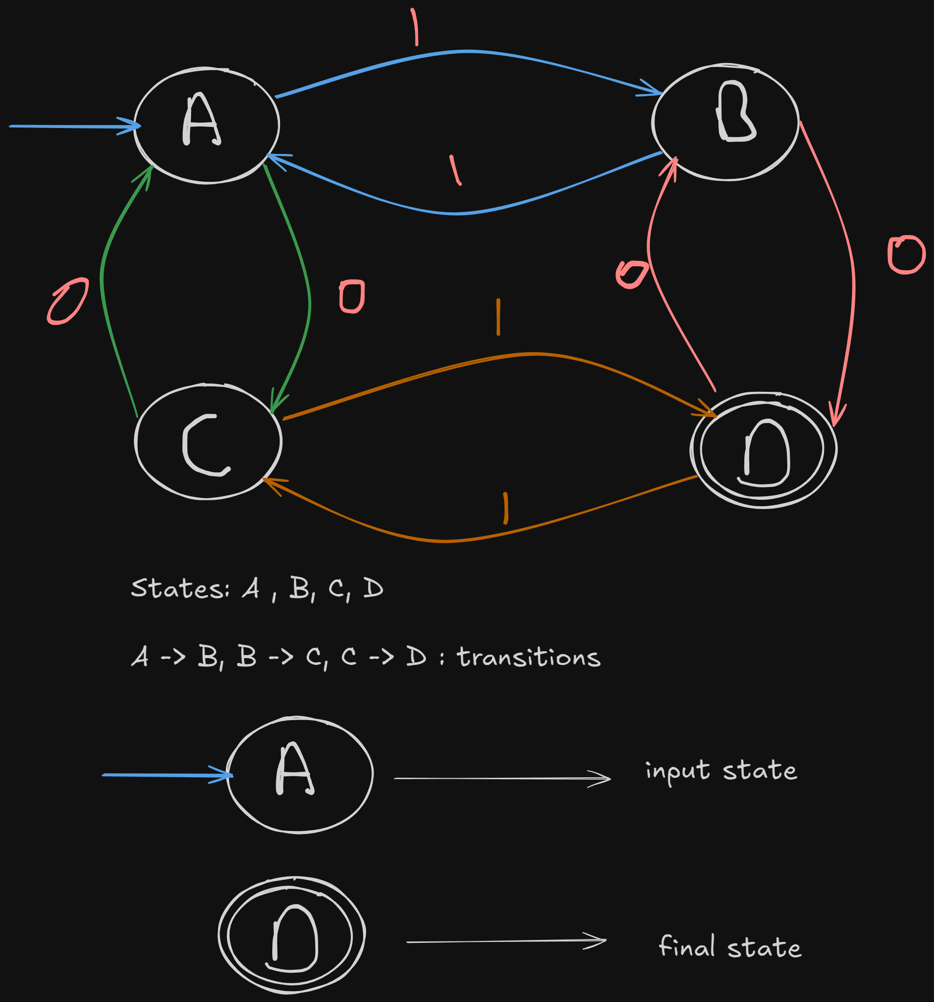
2. Non-deterministic Finite Automata (NFA)
“Parallelism, Randomness”
“multiple next states, could be chosen at random”.
A simple difference between an NFA and a DFA
Example
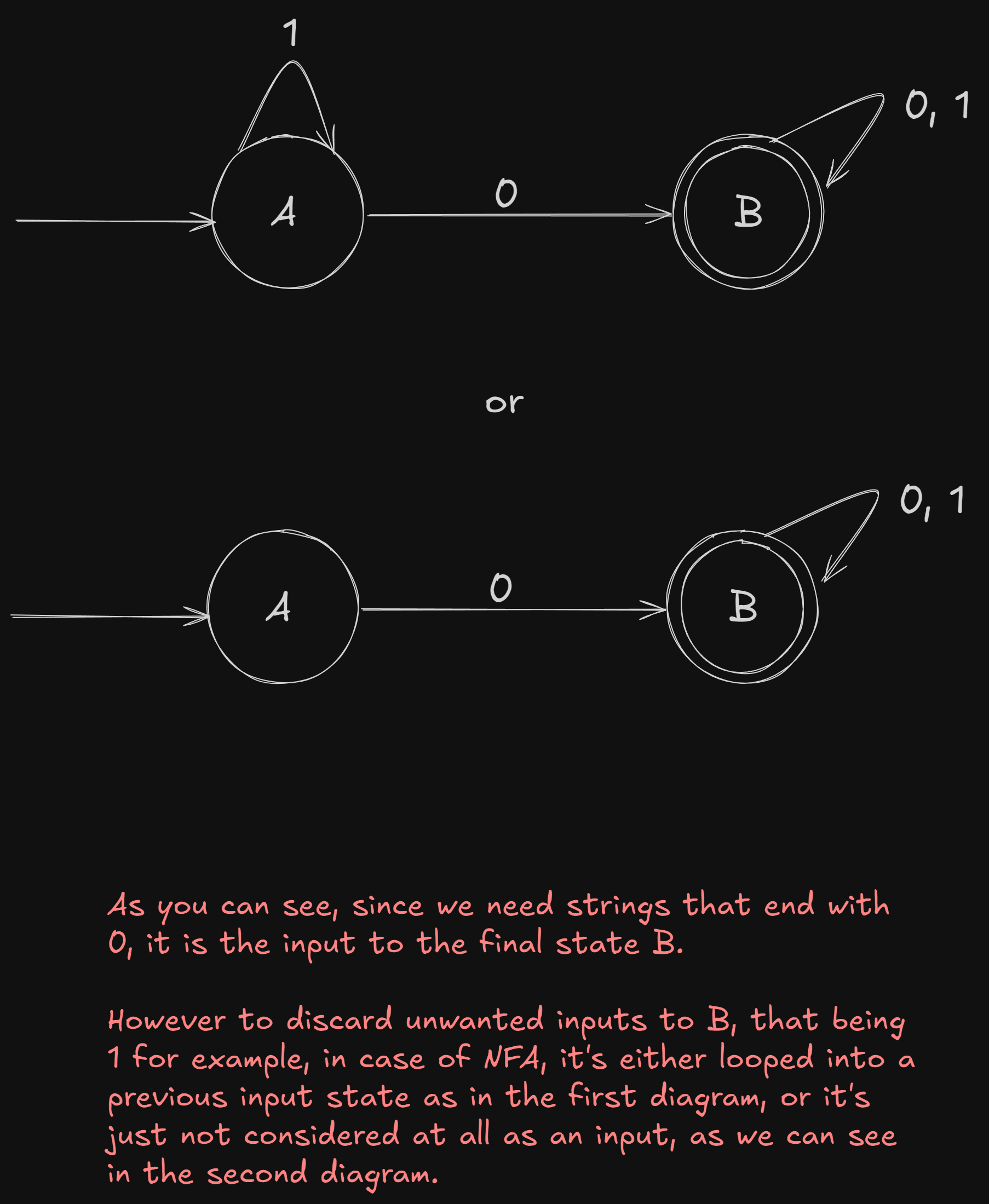
Construct a finite automata for this language :
DFA implementation
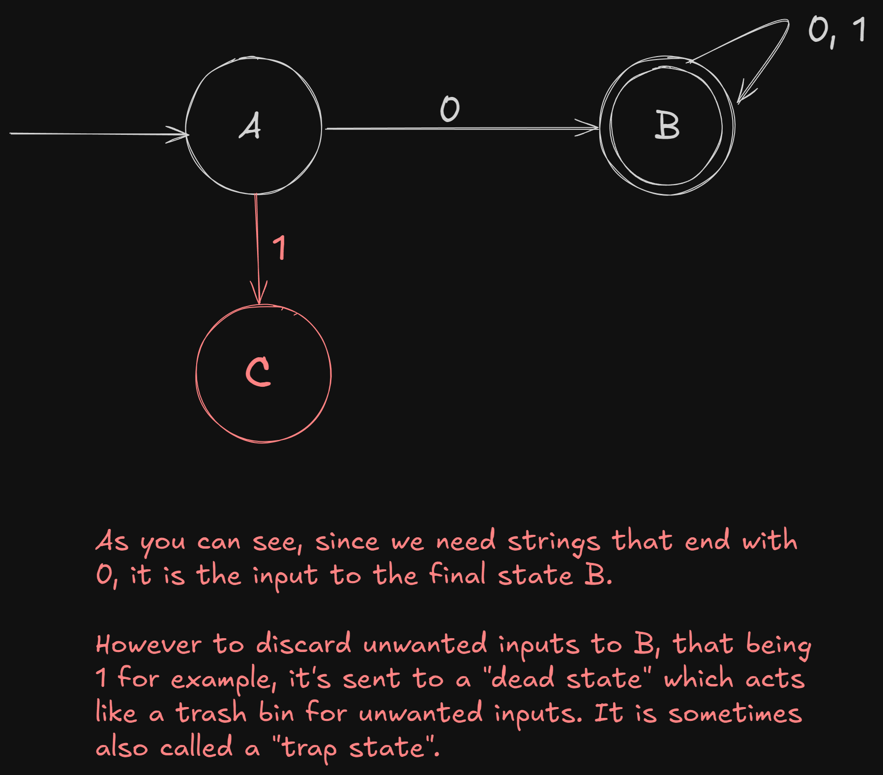
NFA implementation
2. NFA to DFA conversion
https://www.youtube.com/watch?v=—CSVsFIDng&list=PLBlnK6fEyqRgp46KUv4ZY69yXmpwKOIev&index=15&pp=iAQB
Converting a DFA to NFA is easy, just remove the dead state and keep the unwanted inputs looped in other states, or don’t.
However the conversion of a NFA to DFA is tedious process.
As

Let’s understand this with an example :
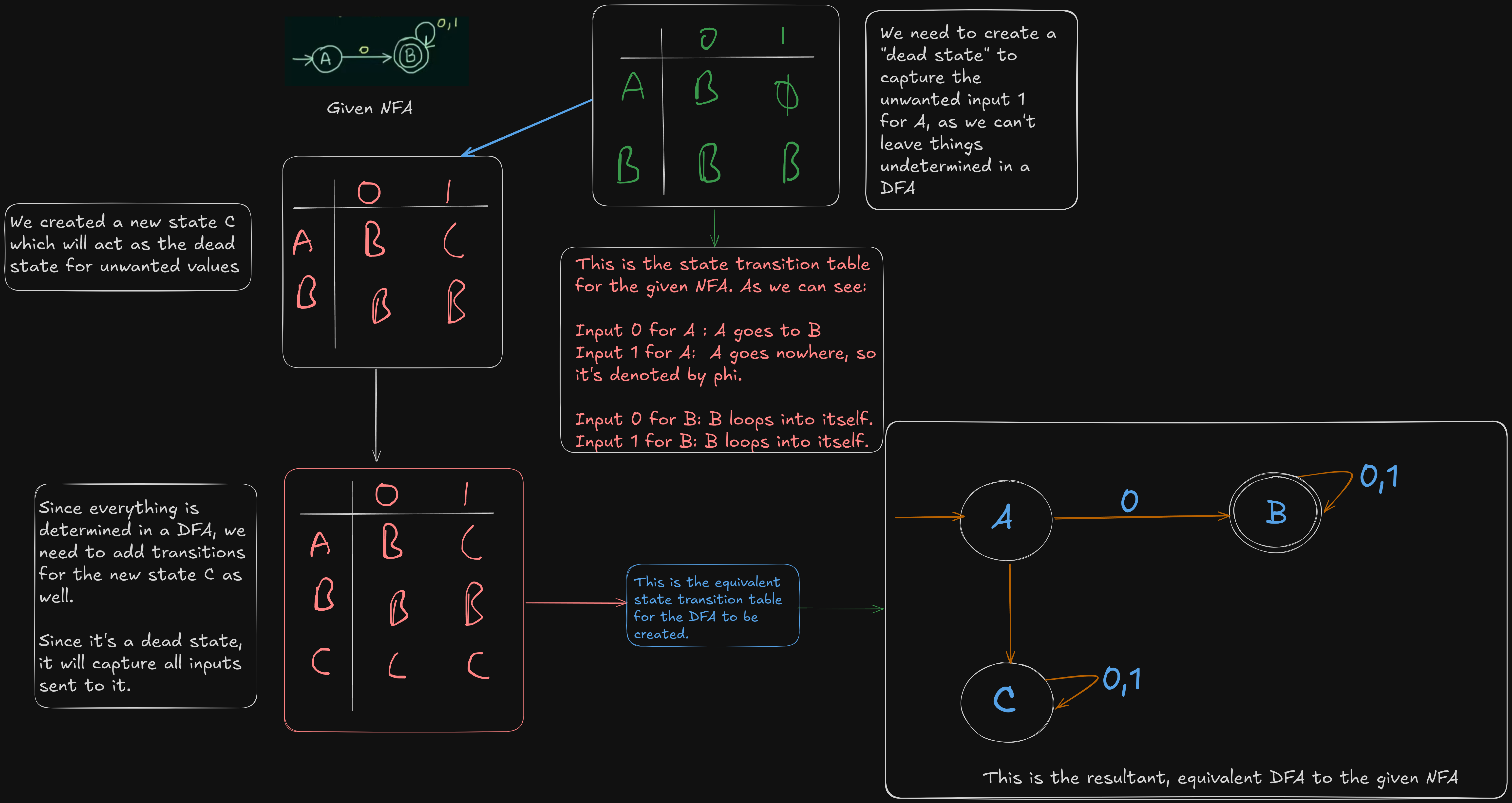
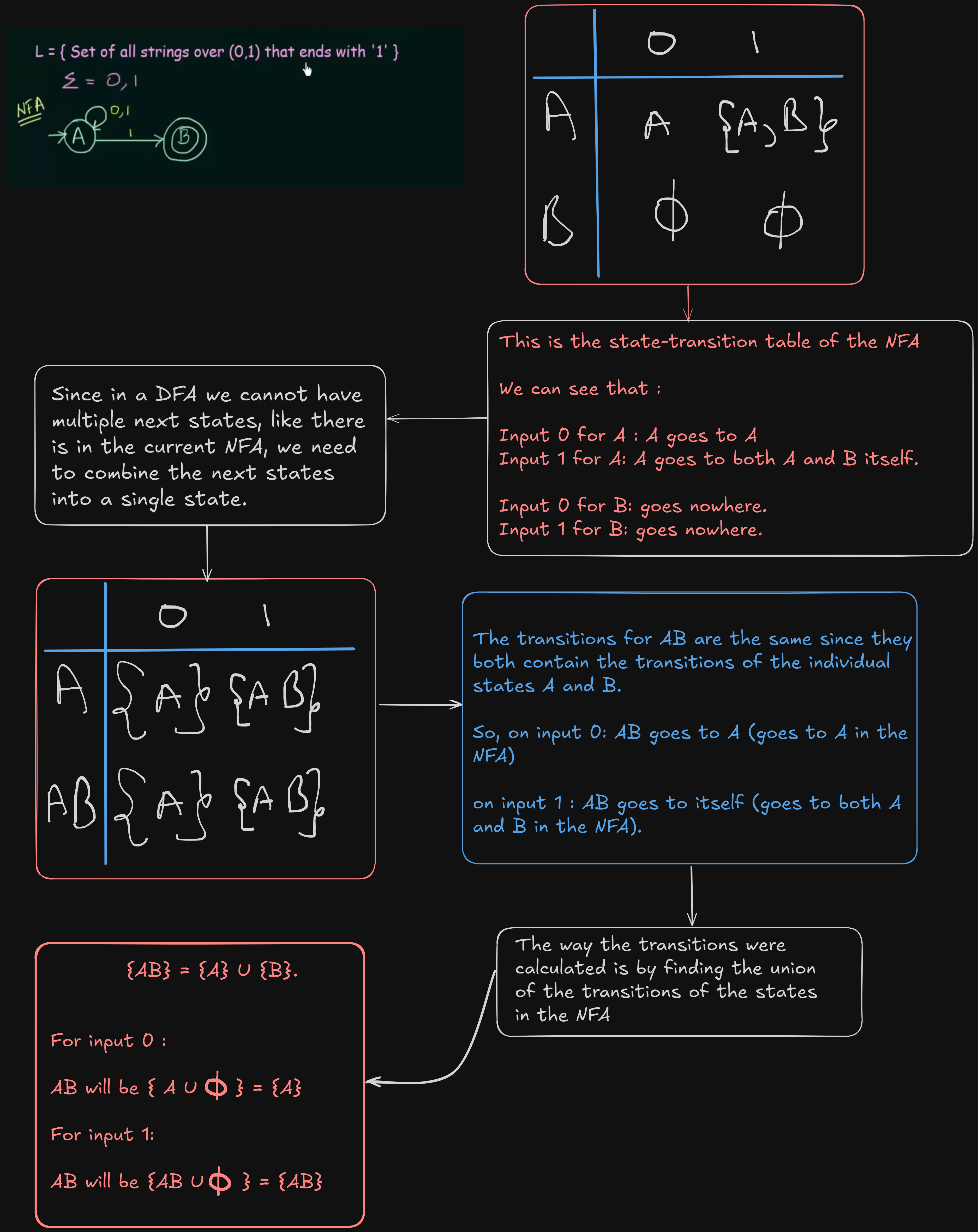
Example 1.

Here we have the given NFA already.
So to convert it to a DFA, we need to construct the state transition table of the NFA, then construct the equivalent table for the DFA.
Example 2 (Very important)
https://www.youtube.com/watch?v=pnyXgIXpKnc&list=PLBlnK6fEyqRgp46KUv4ZY69yXmpwKOIev&index=16
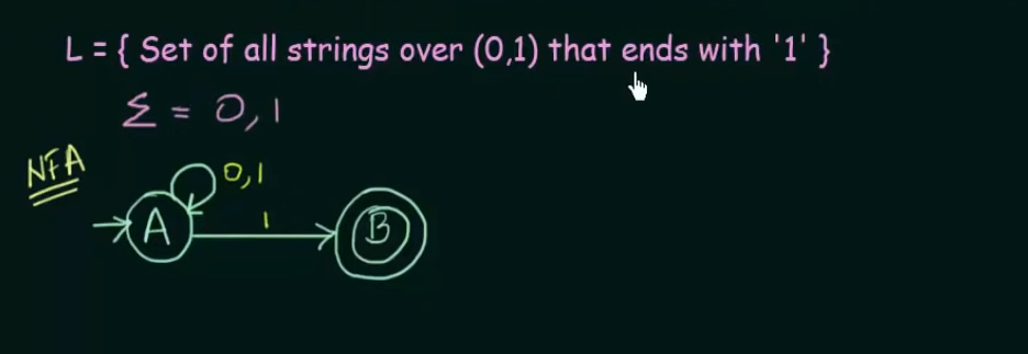
So here we have the NFA already constructed.
Thus, the resultant DFA will be :

3. Minimization of DFA
https://swaminathanj.github.io/fsm/dfaminimization.html

So here we will use Hopcroft’s algorithm to minimize a DFA.
Hopcroft’s algorithm is based on Myhill-Nerode equivalence relation that splits the states into a group of equivalent classes. A set of states belong to the same class provided they exhibit the same behavior.
Step 1: To start with, we partition the states into two classes.
- Partition 1 groups all states that are final.
- Partition 2 groups all states that a non-final.
In other words, we hypothesize that all the final states may possibly exhibit same behavior and all non-final states may exhibit same behavior.
Step 2: Next, we check if all the states in the same partition exhibit the same behavior.
Definition: Two states are said to be exhibiting the same behavior if and only if for each input, both the states makes transitions to the same partition (not necessarily the same state).
If it is not so, the partition needs to be broken down further and the states are reassigned to different partitions according to their behavior.
Step 3: Re-compute the transitions with respect to the modified partition set.
Steps 2 and 3 are repeated until
- Either the states in each partition exhibit consistent behavior or
- The partitions have exactly one state and cannot be broken further
Example 1
https://www.youtube.com/watch?v=0XaGAkY09Wc&list=PLBlnK6fEyqRgp46KUv4ZY69yXmpwKOIev&index=21
So let’s work with this example DFA that we have :
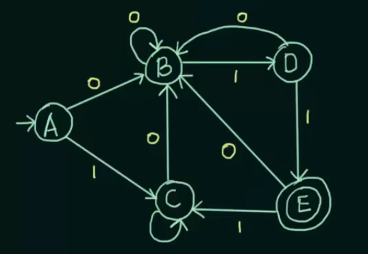
So first of all we will construct the state transition table :
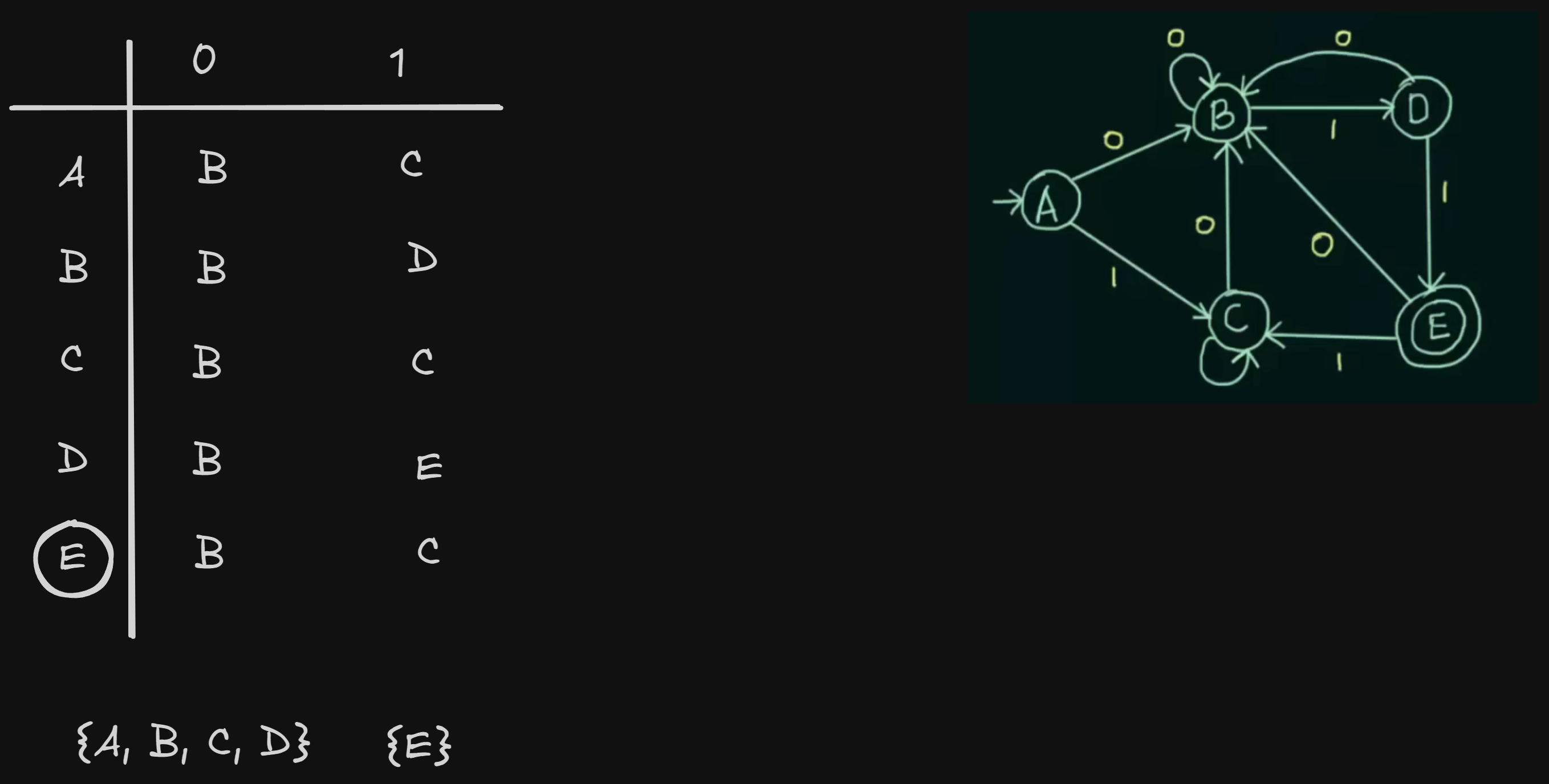
So we have two sets, one having all the non-final states, and the other containing the final states.
So we see for input 0,
A and B share the same next state, but not for input 1. A goes to C and B goes to D.
For input 0,
C and D share the same next state, but not for input 1. C loops to itself while D goes to E.
So we see that both A and C share the same next states for both the inputs.
So A and C can be grouped together.
So we can get new sets :
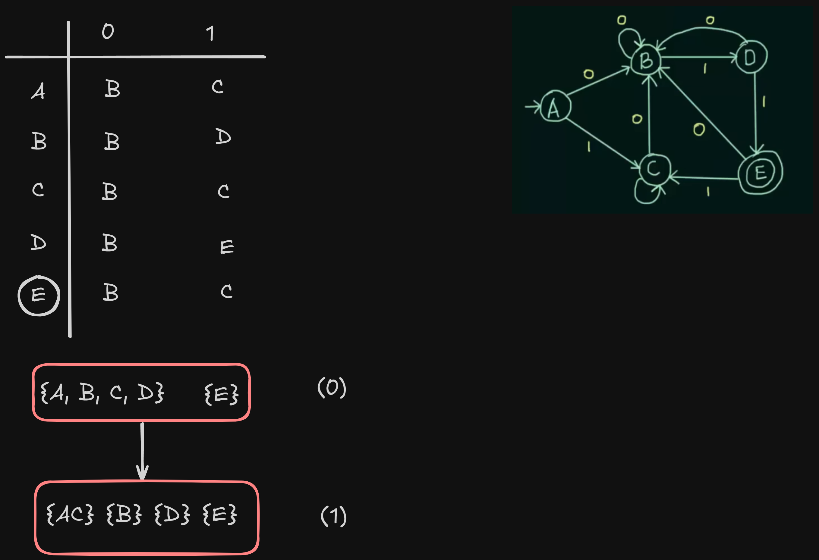
States B and D are separated as well since they don’t share the same next states for both the inputs.
And E stays separated as it is a final state.
Now, to construct the newly minimized DFA, we need to construct the new state transition table.
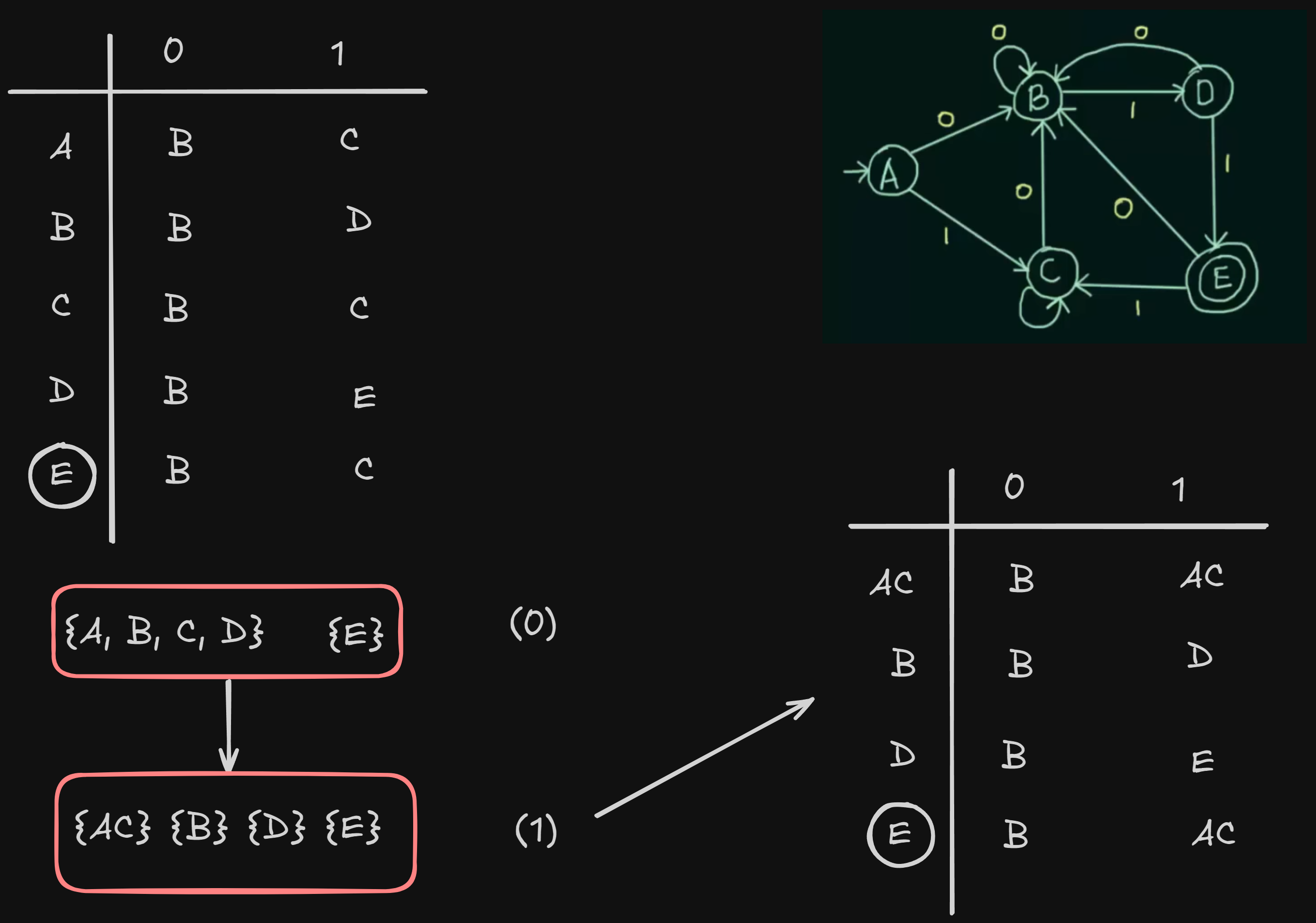
where AC is the new merged state and all independent transitions going to C previously, now go to AC.
So the new DFA will be :
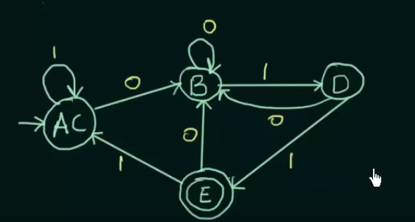
Here are three more example videos on the same topic :
https://www.youtube.com/watch?v=ex9sPLq5CRg&list=PLBlnK6fEyqRgp46KUv4ZY69yXmpwKOIev&index=22&pp=iAQB
https://www.youtube.com/watch?v=DV8cZp-2VmM&list=PLBlnK6fEyqRgp46KUv4ZY69yXmpwKOIev&index=23&pp=iAQB (Minimizing a DFA with multiple final states)
https://www.youtube.com/watch?v=kYMqDgB2GbU&list=PLBlnK6fEyqRgp46KUv4ZY69yXmpwKOIev&index=24&pp=iAQB ((Minimizing a DFA with unreachable states))
Flat recap : Context Free Grammar
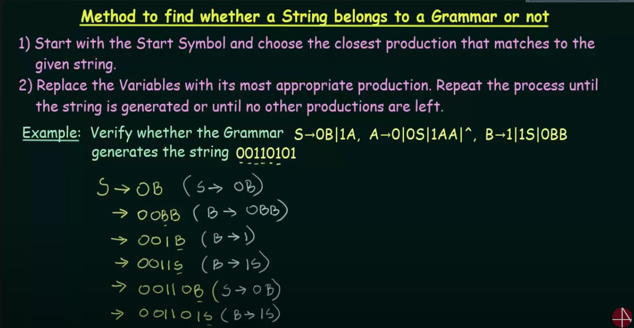
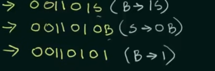
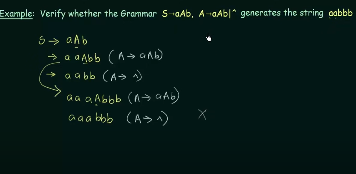
Context Free Language
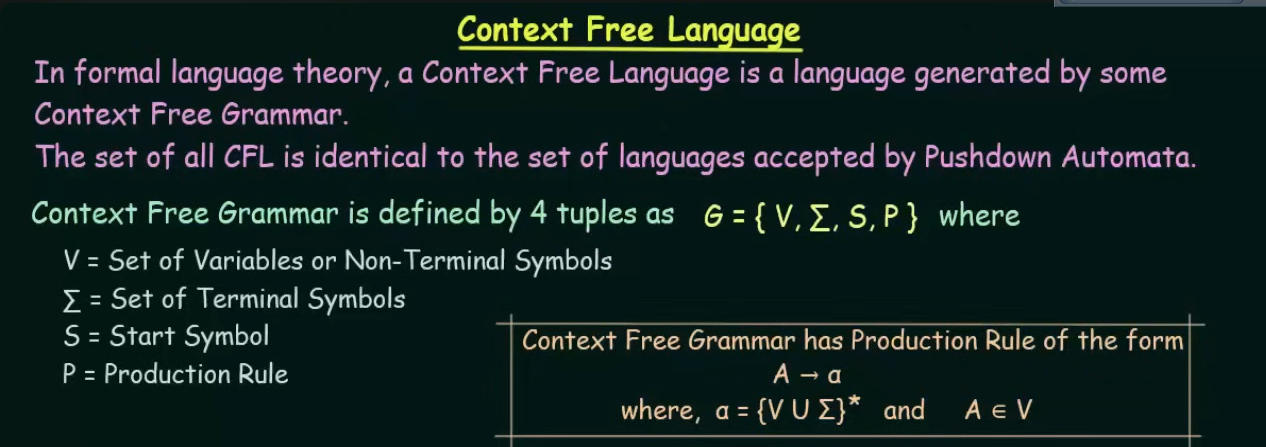
The main difference between CFL and a Regular language is that of the production rule. In RL the production rule is not an iteration, that is, it cannot contain an empty symbol.
However in a CFL the production rule is a closure, that is it can contain an empty symbol.
Example

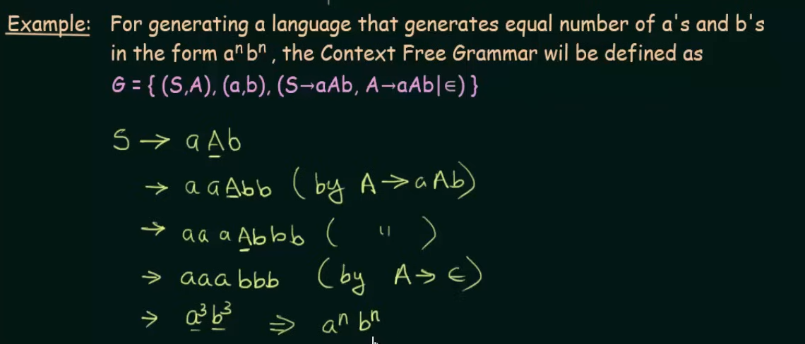
https://www.youtube.com/watch?v=htoFbcwES28&list=PLBlnK6fEyqRgp46KUv4ZY69yXmpwKOIev&index=72
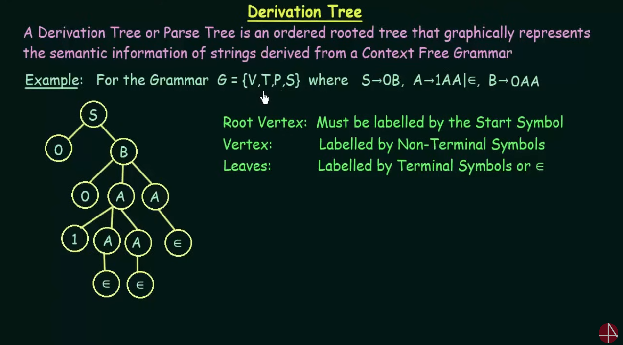
Derivation Tree
https://www.youtube.com/watch?v=u4-rpIlV9NI&list=PLBlnK6fEyqRgp46KUv4ZY69yXmpwKOIev&index=73
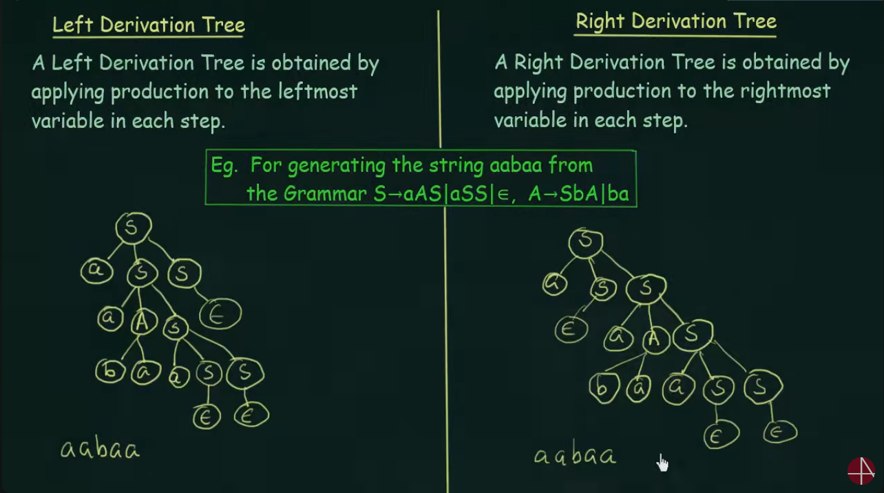
Ambiguous Grammar
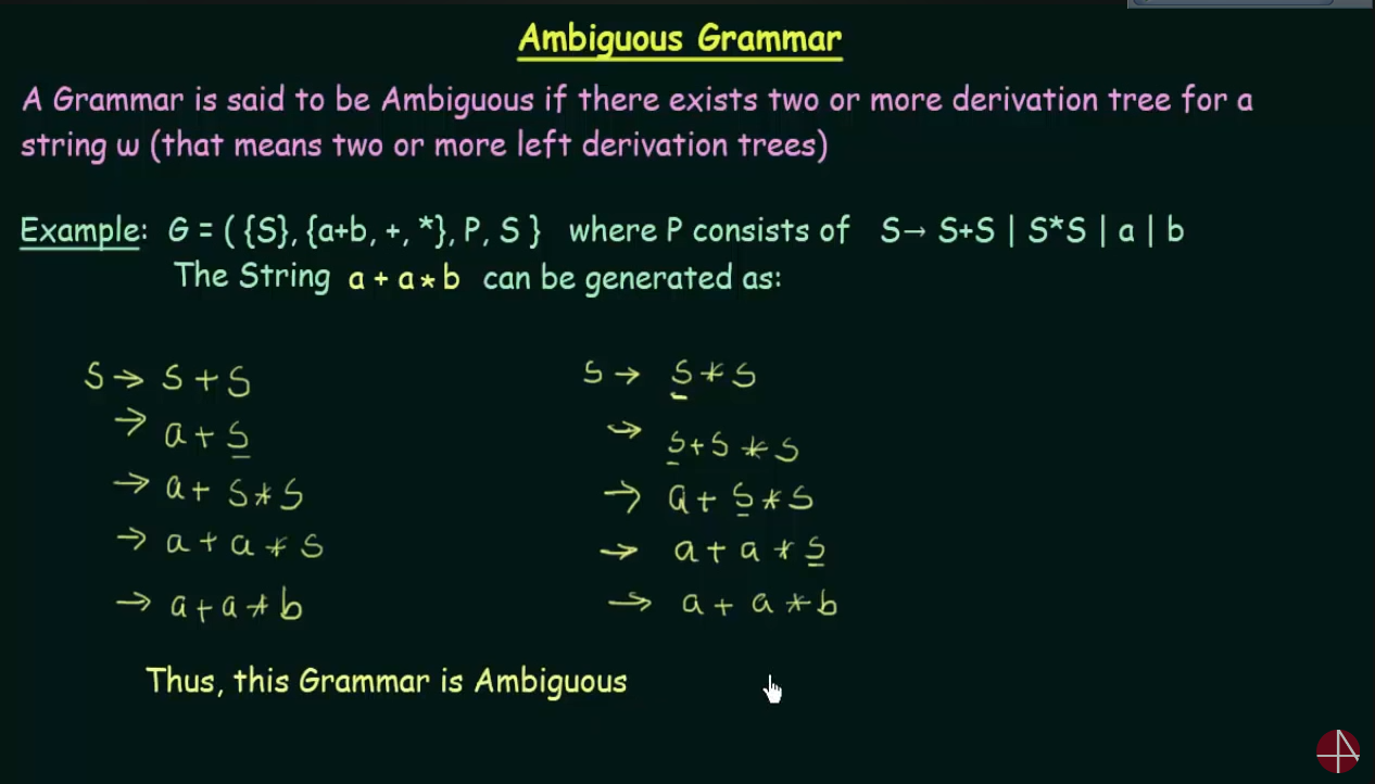
Here instead of drawing a tree, the variables were used on the left and right side respectively.
Reduction/Simplification of Context-Free Grammar
1. Reduction of CFG
https://www.youtube.com/watch?v=EF09zxzpVbk&list=PLBlnK6fEyqRgp46KUv4ZY69yXmpwKOIev&index=78
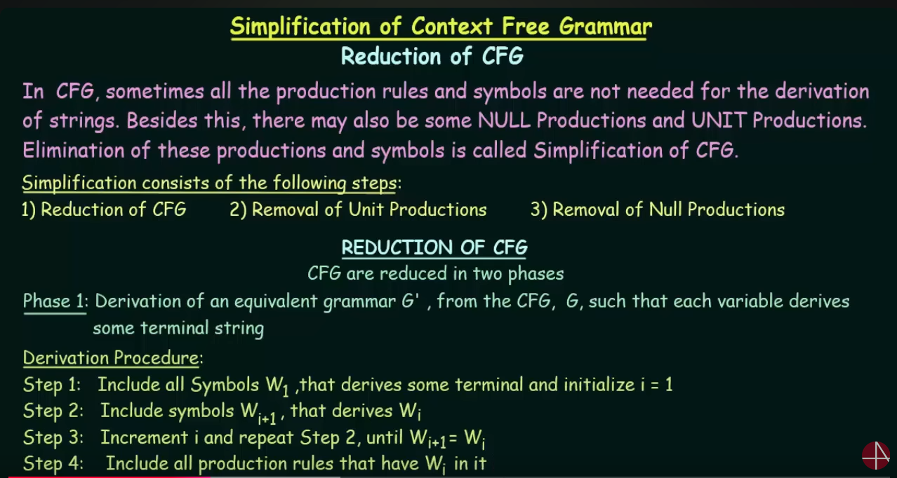

Let’s work this out using an example:

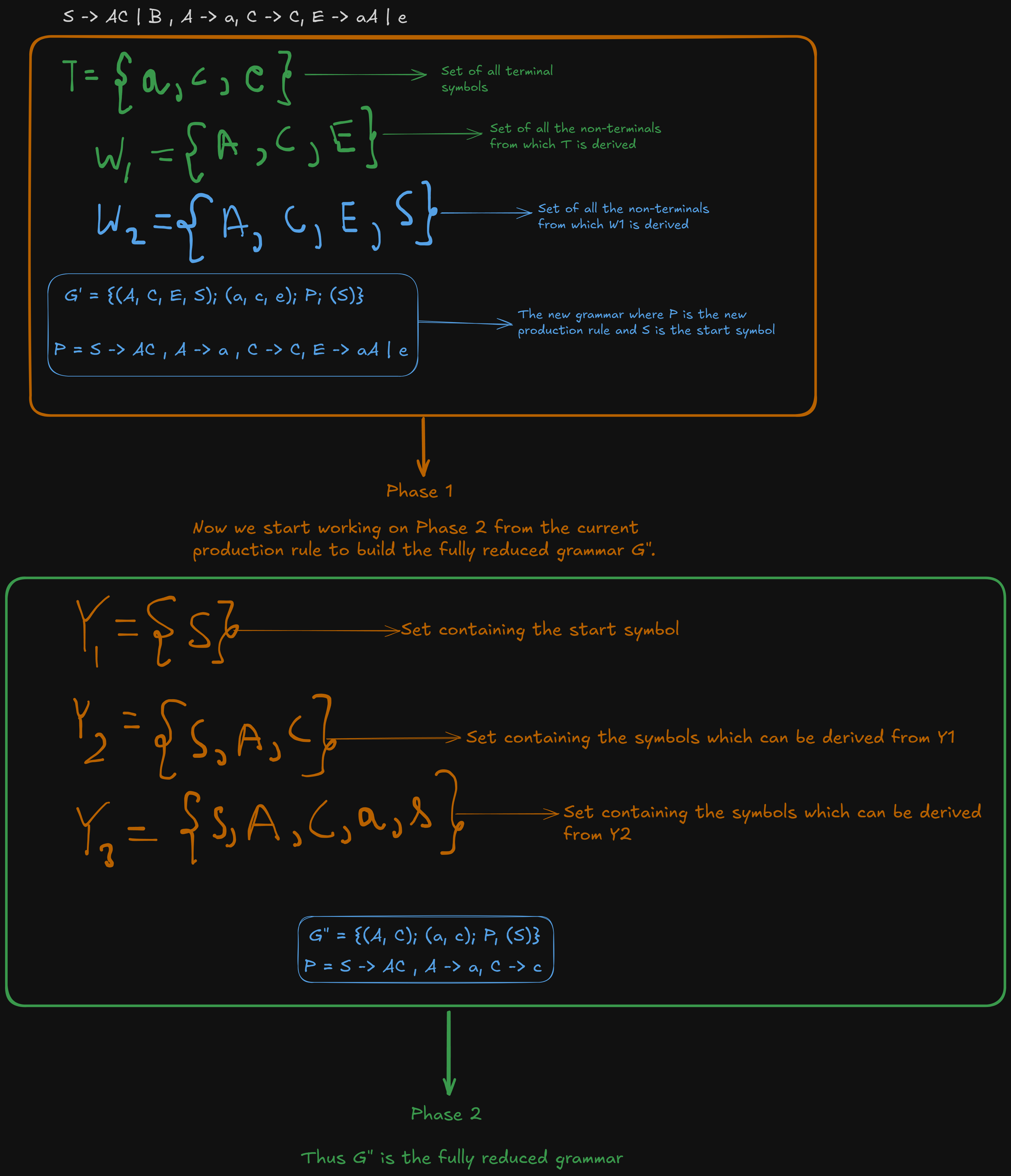
2. Removal of Unit Production
https://www.youtube.com/watch?v=B2o75KpzfU4&list=PLBlnK6fEyqRgp46KUv4ZY69yXmpwKOIev&index=76
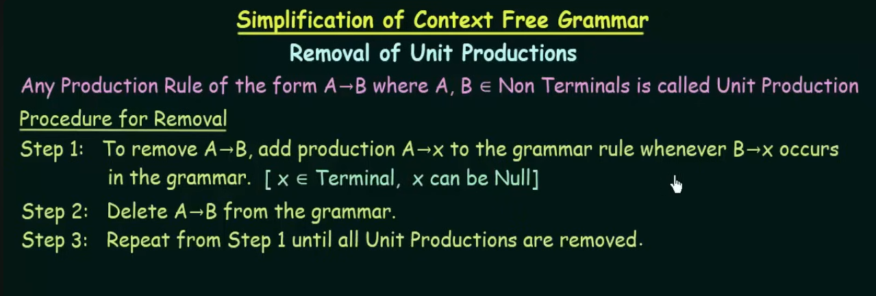
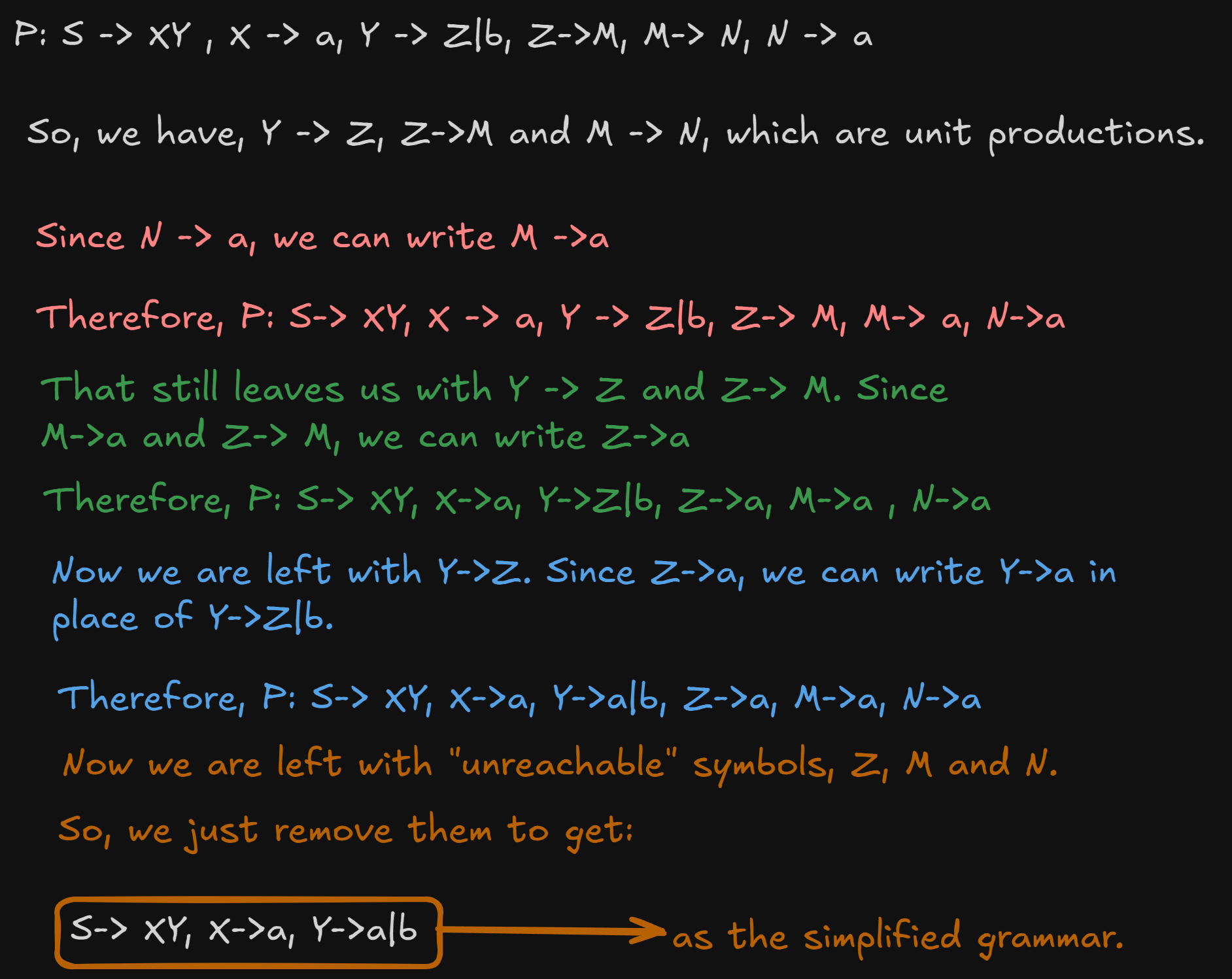
Let’s understand this using an example.

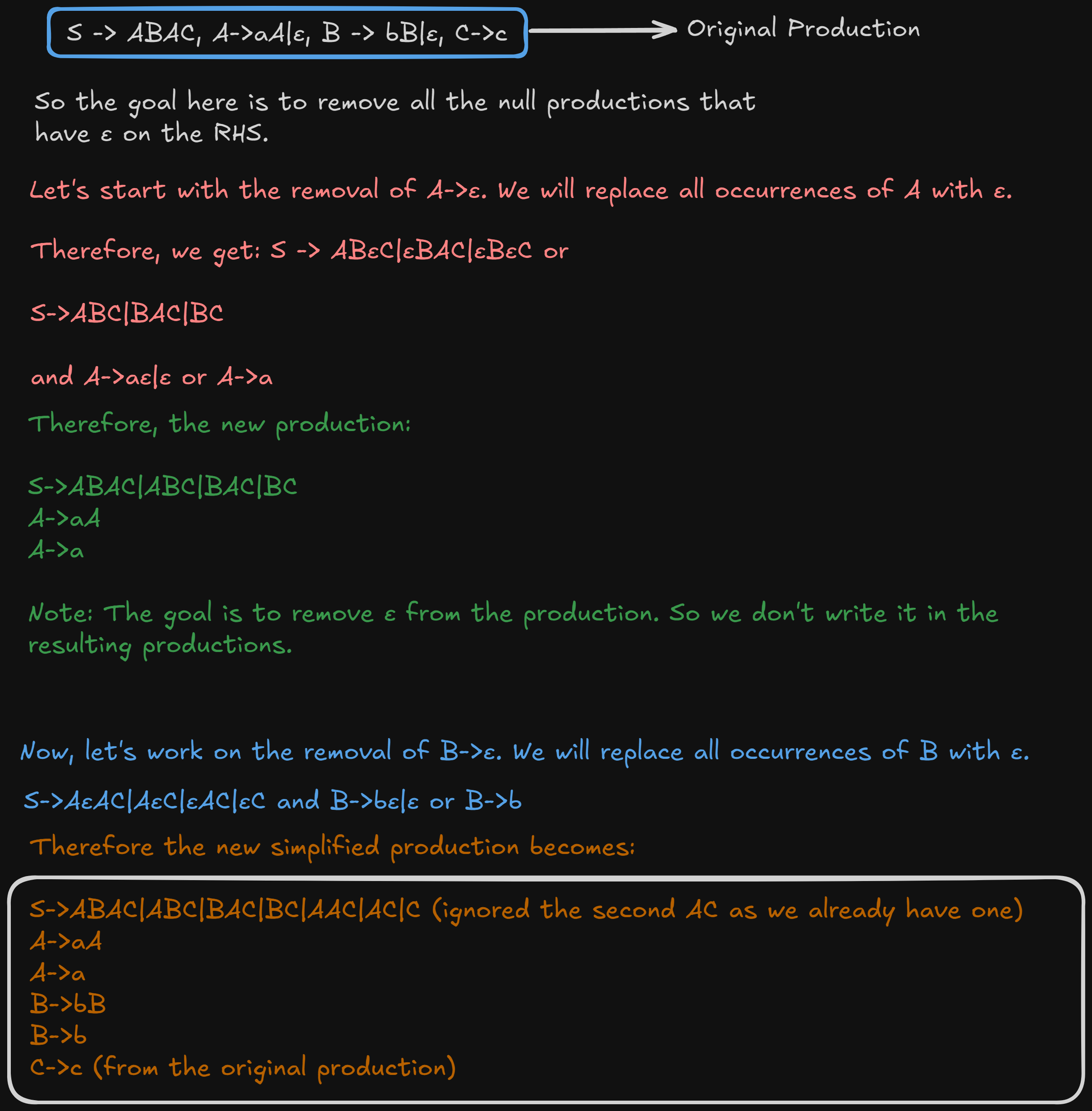
3. Removal of Null Productions
https://www.youtube.com/watch?v=mlXYQ8ug2v4&list=PLBlnK6fEyqRgp46KUv4ZY69yXmpwKOIev&index=77


4. Removal of Left Recursions
This happens during the conversion of Chomsky Normal Form to Greibach Normal Form.
We don’t have the conversions in this semester anymore.
But there was one question regarding the removal of left recursion from a grammar in last year’s (2023) paper.
So I will cover this part.
Still here’s the link for the video where the original production was given in case someone wants to view it
https://www.youtube.com/watch?v=ZCbJan6CGNM&list=PLBlnK6fEyqRgp46KUv4ZY69yXmpwKOIev&index=80&pp=iAQB
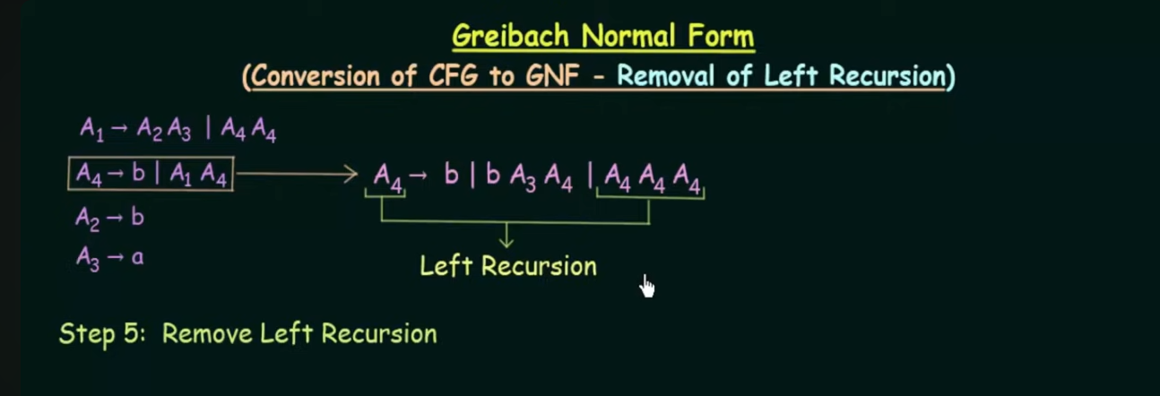
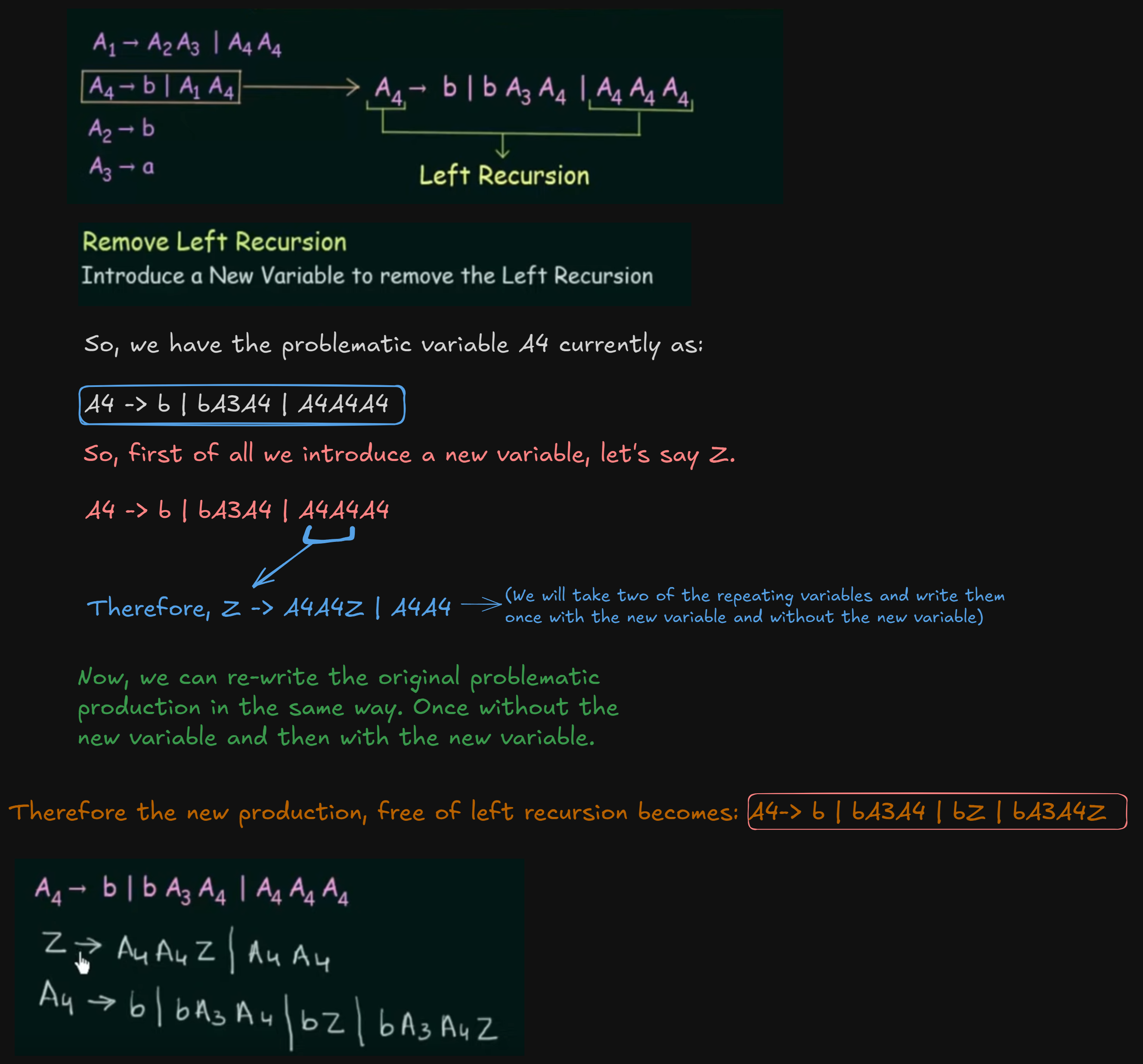
So this is how a left recursion looks.
When the start symbol on the LHS keeps repeating endlessly on the RHS, it’s called a left recursion.
