Fundamental Algorithmic Strategies -- Design and Analysis of Algorithms -- Module 2

---

1. Brute-Force and :

---

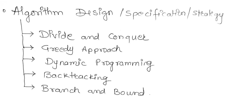
Brute Force

Brute Force is a method of programming in which the algorithm is designed to execute similar or different tasks repeatedly till the goal is achieved. For example brute force programming technique is used in cybersecurity for password cracking in which a large sequence of combinations is repeatedly used on a password protected lock till the lock is opened.

---

Divide and Conquer

The divide and conquer approach involves breaking down a problem into smaller, independent subproblems, solving each subproblem recursively and then combining their solutions to solve the original problem.

Algorithms under divide and conquer approach

1. Binary Search
2. Quick Sort
3. Merge Sort

1. Binary Search

In binary search, an element is searched in an array of elements using a different strategy from Linear search. In binary search, the array is divided into two parts, containing an element in the middle called mid . If the element to be searched is lesser than mid, then the searching is done in the LHS of the array. Else the searching is done in the RHS of the array. This process happens in each recursion call till the element is found.

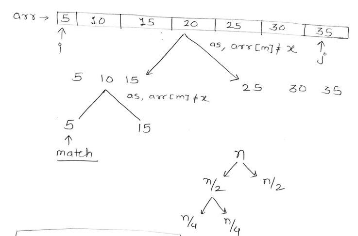
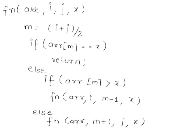
Time complexity : O(n) — Best case O(log n) —Average/Worst Case

---

2. Quick Sort

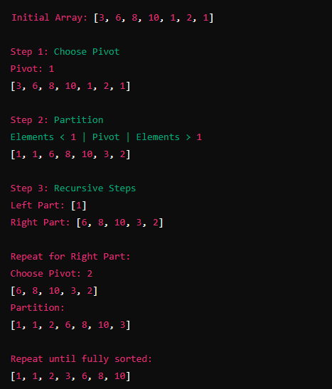
It is another Divide and Conquer algorithm that works by a selecting a pivot element from the array and partitioning the other elements into two sub arrays according to whether the element is greater or lesser than the pivot.

Steps to perform Quick Sort:

• Choose a Pivot: Select an element from the array to be the pivot. The choice of pivot can vary; common strategies include picking the first element, the last element, the middle element, or a random element.
• Partition the Array: Reorder the array so that all elements less than the pivot come before it, and all elements greater than the pivot come after it. The pivot is now in its final sorted position.
• Recursively Apply: Recursively apply the same process to the sub-arrays formed by splitting the array at the pivot.

Time Complexity

The time complexity of Quick Sort depends on the pivot selection and partitioning:

1. Best Case: O(n log n)

   • Occurs when the pivot always divides the array into two nearly equal halves.

2. Average Case: O(n log n)

   • On average, the pivot will not divide the array into equal parts, but it will be close enough for the algorithm to run in logarithmic time.

3. Worst Case: O(n^2)

   • Occurs when the pivot is the smallest or largest element every time, causing the array to be divided into one empty sub-array and one sub-array with n-1 elements.

---

Merge Sort

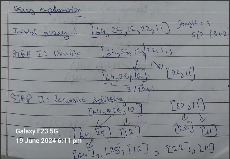
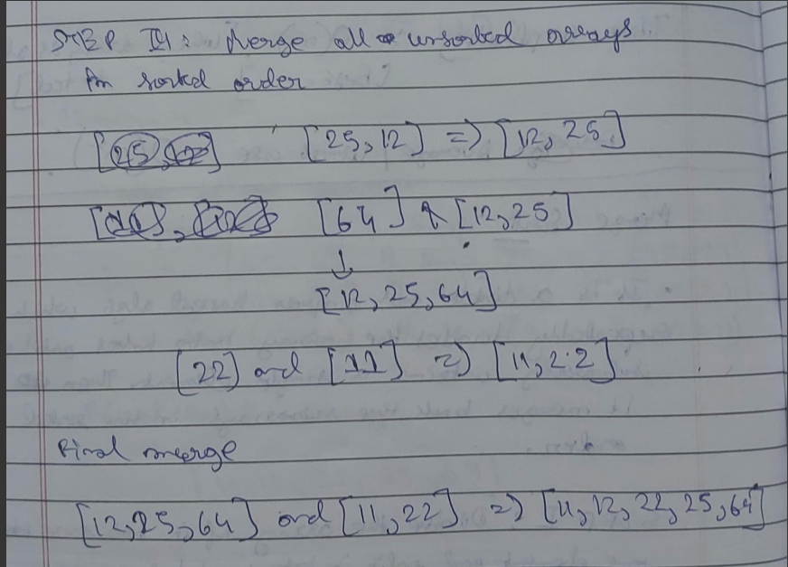
It is a divide and conquer based algorithm which repeatedly divides the array into halves until each half contains just a single element from the original array. The algorithm then works on rearranges the halves in ascending order then rejoins them back into a single array.

Steps for Merge sort:

1. Divide the array if it has more than one element and split it into two halves.
2. Recursively sort each half.
3. Combine the sorted halves back into a single sorted array.

Time Complexity

Best/Average/Worst Case: O(nlogn)

---

Greedy Programming

Greedy Programming builds up a solution piece by piece, always choosing the next piece that offers the most immediate benefit (i.e., the one that looks the best at the moment). It makes a series of locally optimal choices in the hope that these choices will lead to a globally optimal solution.

Examples:

• Fractional Knapsack Problem.
• Job Sequencing Problem with deadlines.
• Huffman Coding.
• Kruskal’s and Prim’s algorithms for Minimum Spanning Tree.
• Dijkstra’s algorithm for Shortest Path in a graph.

1. Fractional Knapsack Problem

Problem Statement: You are given a set of of items, each with a weight and value. You have a knapsack with a max weight capacity. The goal is to maximize the total value of the items in the knapsack without exceeding the weight capacity.

In this fractional knapsack problem, you are allowed to take fractions of items, meaning we can break items into smaller parts and take those smaller parts into a knapsack in case adding the entire item will exceed the max capacity of the knapsack.

Steps for this algorithm :

Initialization

Start with an empty knapsack with a total value of 0.

Selection

Calculate the value-to-weight ratio for each item. Sort the items in descending order based on their value-to-weight ratio.

Feasibility check and Incorporation

1. Iterate through the sorted list of items.
2. For each item, check if the entire item can fit into the knapsack without exceeding capacity.
3. If yes, then add the total value of the item to the knapsack and decrease the total capacity of the knapsack by the weight of the item.
4. If no, then take the fraction of the item into into the remaining capacity, add the corresponding value to the total value, and fill the knapsack to it’s full capacity.
5. Repeat till knapsack is full/no items are left.

Example

• Items and Their Values: You have a set of items, each with a weight and a value. For example, let’s say you have 3 items:

  • Item 1: weight = 10, value = 60
  • Item 2: weight = 20, value = 100
  • Item 3: weight = 30, value = 120

• Knapsack Capacity: The knapsack has a maximum weight capacity, say 50.

• Value-to-Weight Ratio: Calculate the value-to-weight ratio for each item. This helps in deciding which item (or fraction of it) to take first. The ratios are:

  • Item 1: 60/10 = 6
  • Item 2: 100/20 = 5
  • Item 3: 120/30 = 4

• Sorting: Sort the items based on their value-to-weight ratios in descending order. So, the order becomes: Item 1, Item 2, Item 3.

• Filling the Knapsack: Start with the item with the highest ratio and add as much of it as possible to the knapsack. If the knapsack can’t hold the entire item, add as much as possible and move to the next item. Repeat this process until the knapsack is full.

  For our example:

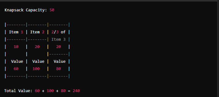
  • Add Item 1 (10 units, value 60), remaining capacity = 50 - 10 = 40.
  • Add Item 2 (20 units, value 100), remaining capacity = 40 - 20 = 20.
  • Add 2/3 of Item 3 (20 units, value 80), remaining capacity = 20 - 20 = 0.

  Total value = 60 + 100 + 80 = 240.

Time Complexity

• Best Case: O(nlog⁡n)
• Average Case: O(nlog⁡n)
• Worst Case: O(nlog⁡n)

---

The Job Sequencing Problem

The Job Sequencing Problem involves scheduling jobs to maximize profit, where each job has a deadline and a profit if completed by its deadline. Each job takes one unit of time, and we cannot extend beyond the maximum deadline.

Steps:

1. Jobs and Their Properties: You have a set of jobs, each with a deadline and a profit. For example, let’s say you have 4 jobs:

   • Job 1: deadline = 4, profit = 20
   • Job 2: deadline = 1, profit = 10
   • Job 3: deadline = 1, profit = 40
   • Job 4: deadline = 1, profit = 30

2. Maximum Deadline: Determine the maximum deadline. Here, it’s 4.

3. Sorting: Sort the jobs based on their profits in descending order. This helps in selecting the most profitable jobs first.

4. Scheduling: Use a slot array to keep track of free time slots and schedule jobs accordingly. Start from the latest possible slot for each job and move backward to find a free slot. If there is no free slot available for a job, then the job is ignored.

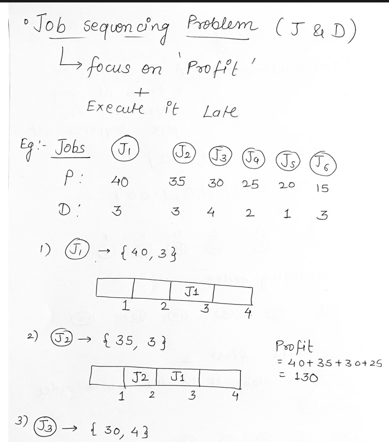
Here even though j4 is set for slot 2, since slot 2 is occupied and slot 1 is free, j4 will be allocated to slot 1 for the maximized profit.

---

Huffman Coding

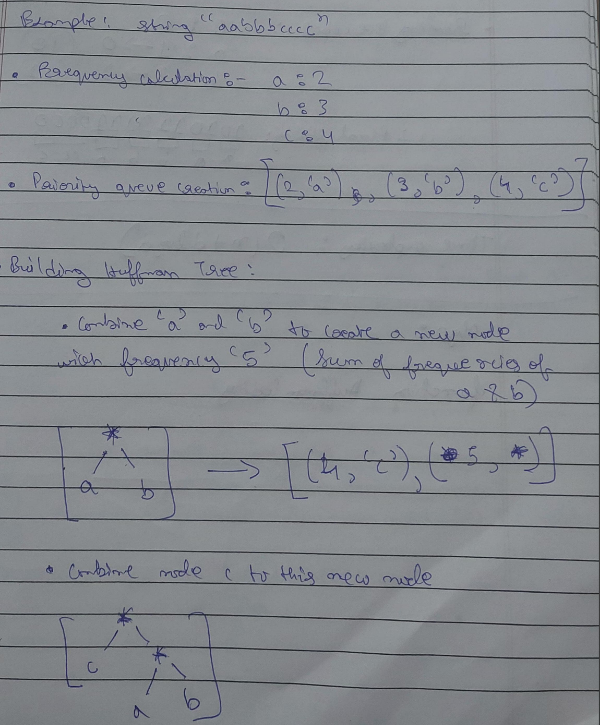
Huffman Coding is a popular algorithm used for lossless data compression. It works by assigning variable-length codes to input characters, with shorter codes assigned to more frequent characters.

Steps for Huffman Coding:

• Frequency Count: Count the frequency of each character in the input data.

• Build a Priority Queue: Create a priority queue (or min-heap) and insert all characters along with their frequencies. Each character is considered as a leaf node.

• Build the Huffman Tree:- While there is more than one node in the priority queue:

  • Remove the two nodes with the lowest frequency.
  • Create a new internal node with these two nodes as children and a frequency equal to the sum of their frequencies.
  • Insert the new node back into the priority queue.
  • The remaining node is the root of the Huffman Tree.

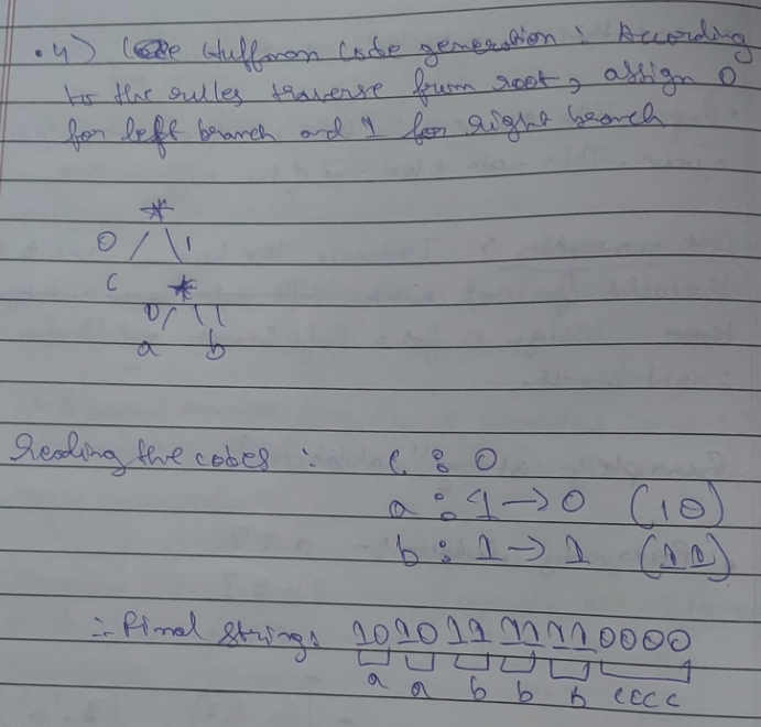
• Assign Codes: Traverse the Huffman Tree to assign codes to characters:

  • Assign ‘0’ for left and ‘1’ for right traversals.

Example

---

Dijkastra’s Algorithm (Shortest Path algorithm)

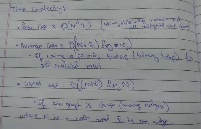
Purpose: Dijkstra’s algorithm is used to find the shortest path from a starting node (also called the source) to all other nodes in a weighted graph.

Step-by-Step Explanation:

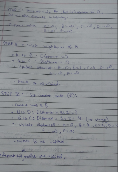
1. Initialization:

   • Start with a graph with nodes and weighted edges (weights represent the distance between nodes).
   • Set the distance to the source node to 0 and all other nodes to infinity.
   • Mark all nodes as unvisited and create a set of all the unvisited nodes.

2. Processing:

   • While there are unvisited nodes:
     1. Select the unvisited node with the smallest distance (let’s call this node u).
     2. For the current node u, consider all its unvisited neighbors. Calculate their tentative distances through u (i.e., the distance to u plus the distance from u to the neighbor).
     3. If the calculated tentative distance is less than the known distance, update the shortest distance to that neighbor.
     4. Mark the current node u as visited (it will not be checked again).

3. Completion:

   • The algorithm completes when all nodes have been visited. The shortest path to each node is now known.

Example

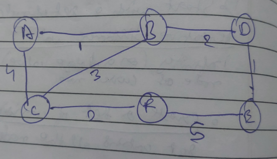
Let’s take this graph

---

Prim’s Algorithm (for finding the Minimum Spanning Tree)

Prim’s Algorithm is used to find the MST of a graph. An MST is a subset of the edges of a connected, undirected graph that connects all the vertices together without any cycles and with the minimum possible total edge weight.

Step-by-Step Explanation:

1. Initialization:

   • Start with any node as the initial node in the MST (let’s call this node u).
   • Mark u as visited.
   • Initialize a priority queue (min-heap) to keep track of the edges connected to the MST.

2. Processing:

   • While there are unvisited nodes:
     1. Select the edge with the smallest weight from the priority queue that connects an already visited node to an unvisited node.
     2. Add this edge to the MST.
     3. Mark the new node as visited.
     4. Add all edges from the newly visited node to unvisited nodes to the priority queue.

3. Completion:

   • The algorithm completes when all nodes are included in the MST.

Example

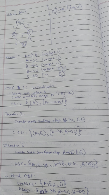
Therefore, total weight = 1+2+3=6.

Time Complexity

• Best Case: O((V+E)log⁡V)
• Average Case: O((V+E)log⁡V)
• Worst Case: O((V+E)log⁡V)

Where V is the number of vertices and E is the number of edges.

---

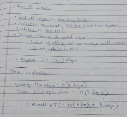
Kruskal’s algorithm.

Kruskal’s algorithm is used to find the Minimum Spanning Tree (MST) of a weighted, undirected graph.

---

Bin Packing (Greedy approach)

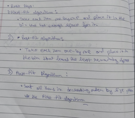
Bin Packing is a way to efficiently pack objects of different sizes into a limited number of containers (bins) of fixed capacity.

The goal is to minimize the number of bins used as much as possible.

Imagine you have a set of items, each with a certain size, and you have bins, each with a fixed capacity. You want to place the items in the bins in such a way that the total size of the items don’t exceed the bin’s capacity.

Example :

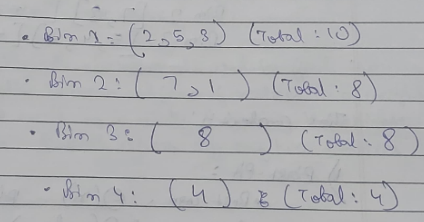
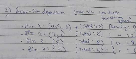
Let there be 4 bins each of capacity 10 & items of sizes : 2,5,4,7,1,3,8

Using First-Fit approach :

Using Best-Fit approach:

Using First-Fit Decreasing approach :

Sort the items into descending order : 8,7,5,4,3,2,1

Bin 1: [8,2] [Space remaining : 0] Bin 2: [7,3] [Space remaining : 0] Bin 3: [5,4,1] [Space remaining: 0]

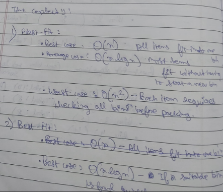
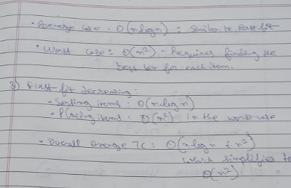
Time complexity :

---

Dynamic Programming

Dynamic Programming (DP) involves breaking a problem into smaller, overlapping subproblems, solving each subproblem just once, and storing their solutions - usually in a table - to avoid redundant computations.

Examples:

• Bellman-Ford Algorithm
• Knapsack Problem (0/1)
• Floyd-Warshall Algorithm

---

Bellman-Ford Algorithm

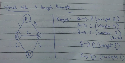
The Bellman-Ford Algorithm is the same as Dijkastra’s algorithm, except that it works for negative edges which Dijkastra’s cannot do so.

The Bellman-Ford Algorithm works by repeatedly relaxing the edges. Relaxation is the process of updating the shortest distance to each vertex by simply visiting it.

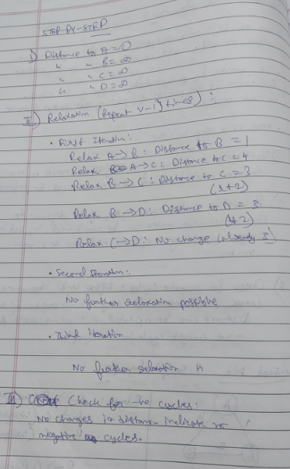
Step-by-Step Explanation

1. Initialization: Start by setting the distance to source vertex as 0 and the distance to the rest of the vertices as infinity.
2. Relaxation: For each edge, if the distance to the destination vertex can be shortened by taking the edge, updating the distance to the destination vertex.
3. Check for negative cycles: After (V-1) iterations, V being the total number of vertices in the graph, check once more for any shorter paths available. If any more distances can be updated, this means there is a negative weight(or more) in the graph.

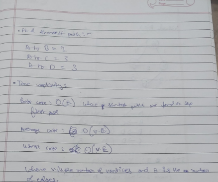
Example

---

0/1 Knapsack Problem (Dynamic Approach)

Warning : This is gonna get big. Had to ask the AI a lot of questions to get thorough explanations.

Imagine you are a thief with a bag (knapsack) that can carry a maximum weight $W$. You have $n$ items to choose from, each with a specific weight and value. Your goal is to maximize the total value of the items in your bag without exceeding the weight limit $W$. The “0/1” part means you can either take an item or leave it (you can’t take fractional parts of an item).

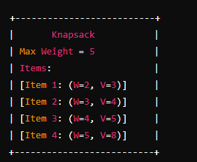
Here’s a simple visual representation:

1. Items: You have items with weights and values.

   • Item 1: Weight = 2, Value = 3
   • Item 2: Weight = 3, Value = 4
   • Item 3: Weight = 4, Value = 5
   • Item 4: Weight = 5, Value = 8

2. Knapsack Capacity: Your knapsack can hold a maximum weight of 5.

W = weight, V = value

How it works

The 0/1 Knapsack problem can be solved using dynamic programming. We’ll create a table where the rows represent items and the columns represent weights from 0 to $W$. The cell $dp[i][w]$ will store the maximum value that can be achieved with the first $i$ items and a total weight of $w$.

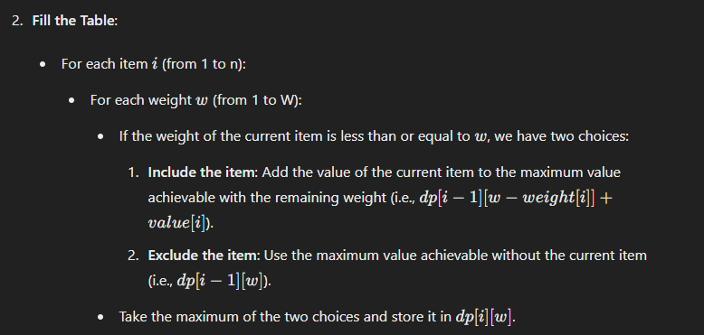
or in simple terms

If we wish to include the item, then we need to add the value of the item to the maximum value (0 initially) to the value of the item.

If we wish to exclude the item then the current maximum value of the knapsack remains as it is.

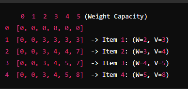
This is the DP (Dynamic Programming) table for the 0/1 Knapsack problem.

How the filling of the DP table works.

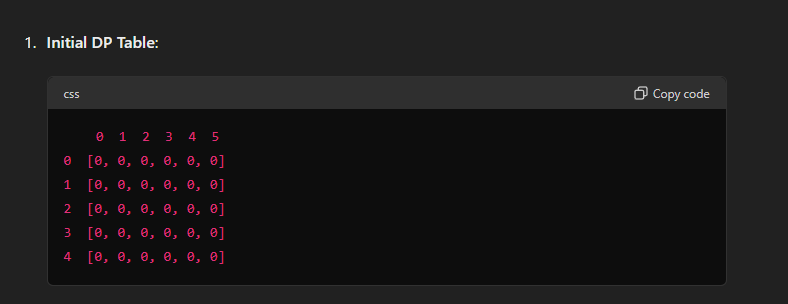
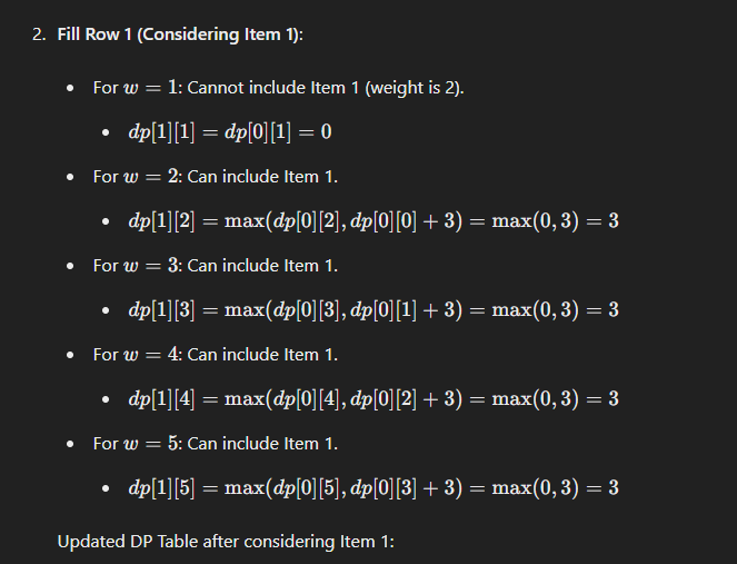
The rule lies in the fact that we cannot enter the items into a position at the table whose weight is lesser than the weight of the item. So we need to find a position in the table where the weight is greater than or equals to the weight of the item.

Thus, we find that at row 1, starting from weight 2, it possible to fill the item all the way till weight = 5

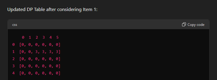
By filling the entire row, we ensure that for each possible weight capacity, we know the maximum value achievable with the items considered so far. This way, when we move to the next item, we can make informed decisions based on the already optimal solutions stored in the DP table.

Now, for the remaining items :

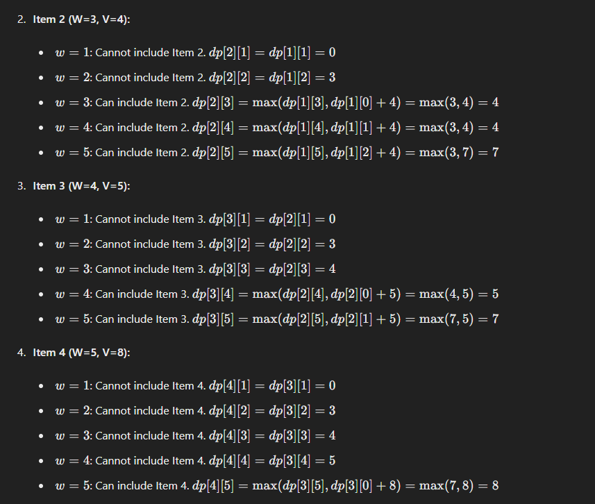Now what is the case of this ''max"?

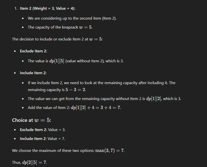
Basically another fancy term of "adding the value of the current item with the value of the given item at the existing weight".

At weight = 5 previously item of value 3 was there. When item of value 4 was considered to be filled at that weight, it was added with the existing value, i.e 3+4 = 7.

Then when we take the ==final decision of including the item of new value 7 and excluding the item of old value = 3,== we take the maximum of the two value and settle on keeping the one with the greater value.

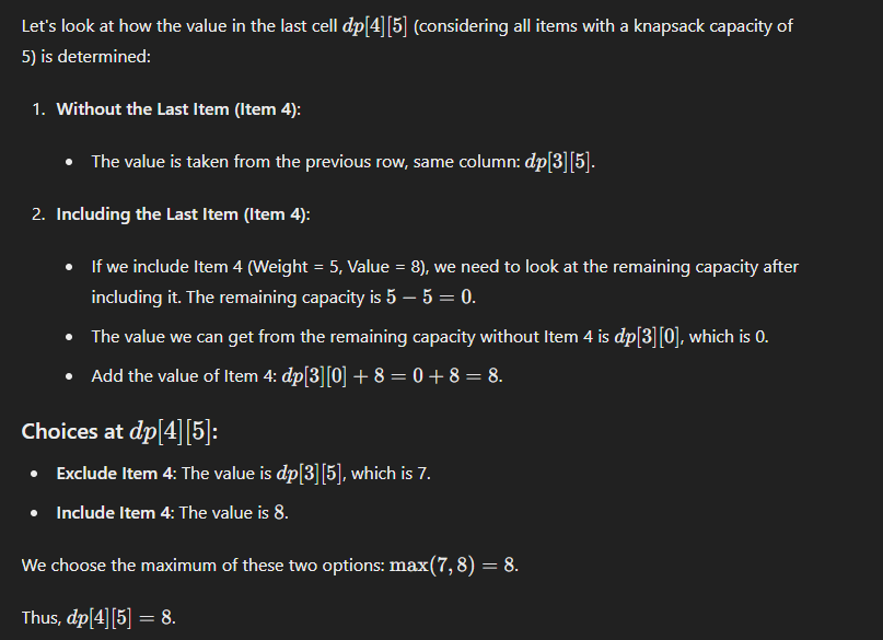
Now one may ask, that by this logic wouldn't the item at the last row and last column of value 8, be added to the previous value of 7 and we get the new value of 15?

But nah, that doesn’t happen.

Why Not Simply Add Values?

The reason we don’t just add the value of the current item to the previous maximum value (resulting in 15) is because each item of the same weight can only be included once. The DP table captures the maximum value for each weight capacity considering all combinations of items without duplication. This ensures that each item’s inclusion is based on valid remaining capacity, preventing the same item from being counted multiple times.

That is why we decided to take the greater value of 8 and remove the lesser value of 7, and not add them, despite the both items having the same weight.

Summary:

• Each item of the same weight can be included only once: This ensures that we don’t exceed the weight capacity or double-count any item.
• Choice of including or excluding an item: For each item and weight capacity, we choose the maximum value achievable by either including or excluding the item.
• DP Table Construction: The table is filled to ensure that each subproblem (defined by items considered and weight capacity) is solved optimally, and these solutions are used to build the solution to the full problem.

Final DP table once again for clarification :

---

The remaining content is continued in the next pdf.