Numerical Methods -- Interpolation -- Module 2

---

Index

1. Interpolation and it’s methods.
2. 1. Newton’s Forward and Backward interpolation methods.
3. The Newton forward interpolation polynomial is written as
4. The Newton backward interpolation polynomial is given by
5. The Lagrange Interpolation Formula
6. 3. Newton’s Divided Difference interpolation

---

Interpolation and it’s methods.

In numerical analysis, interpolation is a method of estimating values within a range of known data points, essentially finding new data points based on the values of a function at a limited number of points.

• The Problem:

  You have a set of data points (x, y) representing a function, but you need to estimate the function’s value at a point that lies between the known data points. 

• The Solution:

  Interpolation uses the known data points to construct a simpler function (like a polynomial or spline) that passes through those points, and then uses this simpler function to estimate the value at the desired point.

Methods of Interpolation

Depending on the interval between the data points, there are different interpolation methods.

Equal Intervals

1. Newton’s Forward and Backward interpolation methods.

Let’s try to understand these methods with an example.

https://www.youtube.com/watch?v=Aw6LvaPtESE&list=PLU6SqdYcYsfLrTna7UuaVfGZYkNo0cpVC&index=5

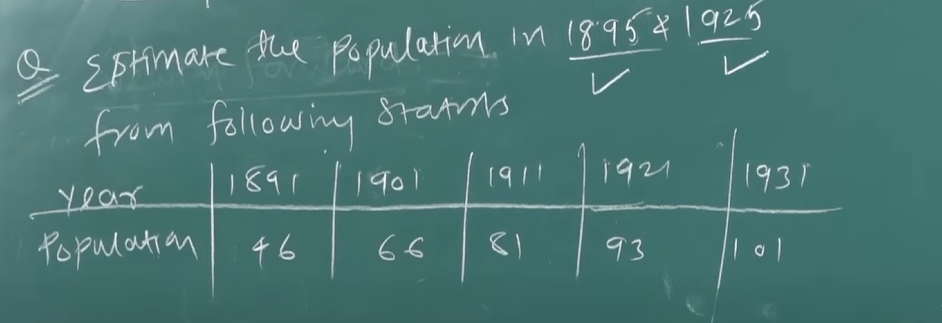
So we have these values given for a 10 year interval.

We will start by tabulating these values.

We set the intervals to x and it’s values list to f(x).

x	f(x)
1891	46
1901	66
1911	81
1921	93
1931	101

The gaps between the cells are intentional, as you will see below.

Now we set the next column to $\Delta f(x)$ and the next to ${\Delta }^{2}f(x)$ and the next to ${\Delta }^{3}f(x)$ and so on…

x	f(x)	$\Delta f(x)$	${\Delta }^{2}f(x)$	${\Delta }^{3}f(x)$	${\Delta }^{4}f(x)$
1891	46
		20
1901	66
		15
1911	81
		12
1921	93
		8
1931	101

Now we find the value of $\Delta f(x)$ by taking the difference of the values of $f(x)$.

So between 1891 and 1901 the value will be given by $66-46=20$

Then between 1901 and 1911 it will be $81-66=15$

And between 1921 and 1911 it will be $93-81=12$

And between 1921 and 1931 it will be $101-93=8$

Now we will populate the values of the other columns similarly

x	f(x)	$\Delta f(x)$	${\Delta }^{2}f(x)$	${\Delta }^{3}f(x)$	${\Delta }^{4}f(x)$
1891	46
		20
1901	66		-5
		15		2
1911	81		-3		-3
		12		-1
1921	93		-4
		8
1931	101

This can keep going on as long as we would like but it’s better to stop at ${\Delta }^{4}f(x)$ for now.

Now there are two formulae for Newton’s Interpolation

---

The Newton forward interpolation polynomial is written as:

$\boxed{P(x)=f(x_0)+p\Delta f(x_0)+\frac{p(p-1)}{2!}{\Delta }^{2}f(x_0)+\frac{p(p-1)(p-2)}{3!}{\Delta }^{3}f(x_0)+\cdots }$

where - Step Size (h):

• Since the nodes are equally spaced, $h=x_1-x_0=x_2-x_1=....$.

• Parameter p:

  • Defined as:

    $p=\frac{x-x_0}{h}$​​

  • This non-dimensional number tells you how far $x$ is from $x_0$​ in terms of the step size.

And :

The Newton backward interpolation polynomial is given by:

$\boxed{P(x)=f(x_n)+p\nabla f(x_n)+\frac{p(p+1)}{2!}{\nabla }^{2}f(x_n)+\frac{p(p+1)(p+2)}{3!}{\nabla }^{3}f(x_n)+\cdots }$

Parameter p:

• For backward interpolation, we define:

  $p=\frac{x-x_n}{h}$​​

• Here, $x_n$​ is the last (largest) $x$-value in your table.

---

Which one to use and when?

That will depend on the given question.

We have been asked to estimate the population between 1895 to 1925

x	f(x)	$\Delta f(x)$	${\Delta }^{2}f(x)$	${\Delta }^{3}f(x)$	${\Delta }^{4}f(x)$
1891	46
		20
1901	66		-5
		15		2
1911	81		-3		-3
		12		-1
1921	93		-4
		8
1931	101

So in this case we need to use Newton’s forward interpolation formula as our range lies between 1891 and 1901.

So we will be using this formula:

$\boxed{P(x)=f(x_0)+p\Delta f(x_0)+\frac{p(p-1)}{2!}{\Delta }^{2}f(x_0)+\frac{p(p-1)(p-2)}{3!}{\Delta }^{3}f(x_0)+\cdots }$

Here $h$ is the step size which is the interval, which is 10 in our dataset.

Now we need to find $p$

Since we are using forward interpolation we use :

$p=\frac{x-x_0}{h}$

Here $x$ is the first end of our required range, i.e 1895.

and $x_0$ is the first entry in the table i.e 1891.

So $p=\frac{1895-1891}{10}$ = $0.4$

And for the first part of the formula we have $f(x_0)$ as 46 from the table.

So $P(1895)=46+0.4\times 20+\frac{0.4(0.4-1)}{2!}\times (-5)+\frac{0.4(0.4-1)(0.4-2)}{3!}\times 2$

$+\frac{0.4(0.4-1)(0.4-2)(0.4-3)}{4!}\times -3$

$=54.8528$

Now for the population of 1925.

We refer to our table again.

x	f(x)	$\Delta f(x)$	${\Delta }^{2}f(x)$	${\Delta }^{3}f(x)$	${\Delta }^{4}f(x)$
1891	46
		20
1901	66		-5
		15		2
1911	81		-3		-3
		12		-1
1921	93		-4
		8
1931	101

We will use Newton’s backward interpolation this time as the range lies towards the end of the table.

So $p=\frac{1925-1931}{10}=-0.6$ Therefore according to the Newton’s Backward interpolation formula

$\boxed{P(x)=f(x_n)+p\nabla f(x_n)+\frac{p(p+1)}{2!}{\nabla }^{2}f(x_n)+\frac{p(p+1)(p+2)}{3!}{\nabla }^{3}f(x_n)+\cdots }$

$P(1925)=101+(-0.6)\times 8+\frac{-0.6(-0.6+1)}{2!}\times (-4)+\frac{-0.6(-0.6+1)(-0.6+2)}{3!}\times (-1)$

$+\frac{-0.6(-0.6+1)(-0.6+2)(-0.6+3)}{4!}\times -3$

$=101-4.8+\frac{(-0.6)(0.4)(-4)}{2}+\frac{(-0.6)(0.4)(1.4)(-1)}{6}+\frac{(-0.6)(0.4)(1.4)(-3)}{24}$

$=96.2-0.48+0.0056+0.042$

$=95.7676$

or we can round to 96 to match with the video

$96.8368$

So we have the population in the years 1895 and 1925 as $54.8528$ and $96.8368$ accordingly.

---

Let’s try out another example

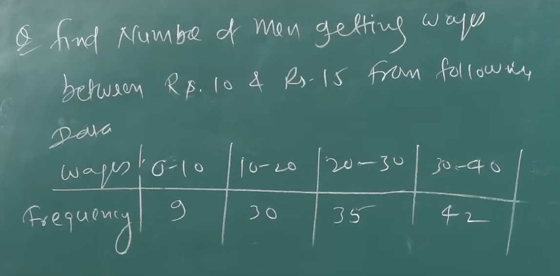
Note that instead of fixed values we have been given ranges for $x$, that represent cumulative frequencies.

So we will construct the table in this way.

Ways (x)	Frequency (f(x))	$\Delta f(x)$	${\Delta }^{2}f(x)$	${\Delta }^{3}f(x)$
Below 10	9
		39 - 9 = 30
Below 20	30 + 9 = 39		35 - 30 = 5
		74 - 39 = 35		7-5 = 2
Below 30	39 + 35 = 74		42 - 35 = 7
		116 - 74 = 42
Below 40	74 + 42 = 116

The reason we added up the values in $f(x)$ was because of the fact that $x$ is given to use as intervals, so the values of $f(x)$ overlap with that of the previous intervals.

And after that it’s just like before, we find the difference to fill up the rest of the columns

Now since we have an interval of 10, so $h=10$

And we are asked to find $f(15)$. Why?

The table represents the cumulative frequency up to wage (not the wage itself) $x$. So $f(10)=9$ means there are 9 men with wages below 10 rupees, $f(20)=39$ means there are 39 men with wages below 20 rupees, and so on.

So if we want to find the number of men getting between wages rupees 10 and 15, we need a number greater than $f(10)$ and less than $f(20)$ .

So $f(15)$ is the best fit here.

So our $x_0$ will be 10 instead of 0

So we will use Newton’s Forward Interpolation formula here

$\boxed{P(x)=f(x_0)+p\Delta f(x_0)+\frac{p(p-1)}{2!}{\Delta }^{2}f(x_0)+\frac{p(p-1)(p-2)}{3!}{\Delta }^{3}f(x_0)+\cdots }$

So $p=\frac{15-10}{10}=0.5$

Now it’s just plain old calculation.

Solving that we should get

$P(15)\approx 24$

Now this is not the final answer yet as we need to find the number of men getting wages between rupees 10 and 15, and since we are given the cumulative frequency and not fixed values, we need to do :

$F(15)-F(10)$

to effectively find the number of men getting wages between rupees 15 and 10.

So that will be $24-9=15$

---

Unequal Intervals

2. Lagrange’s Interpolation for Unequal intervals

Lagrange’s Interpolation is a versatile polynomial interpolation method that works well even when the data points are not equally spaced. Unlike Newton’s formulas, it does not require the data to have equal intervals, and it directly constructs the polynomial that exactly fits the given points

The Lagrange Interpolation Formula

Given a set of n+1n+1n+1 data points:

$(x_0,y_0),(x_1,y_1),\dots ,(x_n,y_n)$,

the Lagrange interpolation polynomial $P(x)$ is given by:

$P(x)={\sum }_{j=0}^n{y}_j{L}_j(x)$

where the Lagrange basis polynomial $L_j(x)$ is defined as:

$L_j(x)={\prod }_{\begin{array}{c}i=0\\ i\ne j\end{array}}^n\frac{x-x_i}{x_j-x_i}$

Key Points:

• Basis Polynomials:
  Each $L_j(x)$ is constructed to be 1 at $x=x_j$​ and 0 at all other data points $x_i$​ (for $i\ne j$). This ensures that when you sum up all terms, $P(x_k)=y_k$ for each $k$.

• Unequal Intervals:
  The formula works for any set of distinct xxx-values, so the spacing between the xxx values does not need to be uniform. Each denominator $x_j-x_i$ adjusts for the actual differences between the points.

---

Looks quite complicated no? Let’s solve this using an example then.

https://www.youtube.com/watch?v=zdyUwzOm1zw&list=PLU6SqdYcYsfLrTna7UuaVfGZYkNo0cpVC&index=4

The first example of this video deals with Lagrange’s Interpolation however the second version deals with Newton’s divided interpolation.

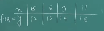
So first off we start with this table

For creating the Lagrange basis polynomial we follow a trick:

So we create pairs first :

$(x_0,y_0)=(5,12)$

$(x_1,y_1)=(6,13)$

$(x_2,y_2)=(9,14)$

$(x_3,y_3)=(11,16)$

So we first “hide” the first $x_0$. And make the first Lagrange polynomial as:

$L_0=\frac{(x-6)(x-9)(x-11)}{}$

And now we put the “hidden” number in place of $x$ in the denominator as:

$L_0=\frac{(x-6)(x-9)(x-11)}{(5-6)(5-9)(5-11))}$

Then we multiply it times it’s $y$ component, in this case $y_0$ which is $12$.

$L_0=(\frac{(x-6)(x-9)(x-11)}{(5-6)(5-9)(5-11))})\times 12$

Similarly we construct the other Lagrange polynomials as well :

We hide $x_1$ or 6

$L_1=(\frac{(x-5)(x-9)(x-11))}{(6-5)(6-9)(6-11)})\times 13$

And for $L_2$

$L_2=(\frac{(x-5)(x-6)(x-11)}{(9-5)(9-6)(9-11)})\times 14$

And for $L_3$

$L_3=(\frac{(x-5)(x-6)(x-9)}{(11-5)(11-6)(11-9)})\times 16$

Now we solve them and add the polynomials

$L_0+L_1+L_2+L_3$

$=\frac{(x-6)(x-9)(x-11)}{(-1)(-4)(-6)}\times 12+\frac{(x-5)(x-9)(x-11)}{(1)(-3)(-5)}\times 13$

$+\frac{(x-5)(x-6)(x-11)}{(4)(3)(-2)}\times 14+\frac{(x-5)(x-6)(x-9)}{(6)(5)(2)}\times 16$

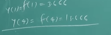
Now, for $x=10$

$=\frac{-4}{-24}\times 12+\frac{-5}{15}\times 13+\frac{-20}{-24}\times 14+\frac{20}{60}\times 16$

$=\frac{12}{6}+\frac{(-13)}{(3)}+\frac{70}{6}+\frac{16}{3}$

$=2-\frac{13}{3}+\frac{35}{3}+\frac{16}{3}$

$=2-\frac{13}{3}+\frac{51}{3}$

$⟹\frac{2}{1}+\frac{38}{3}=\frac{6+38}{3}=\frac{44}{3}$

Final Answer

$\boxed{y(10)\approx 14.666666667}$

---

Let’s try another example

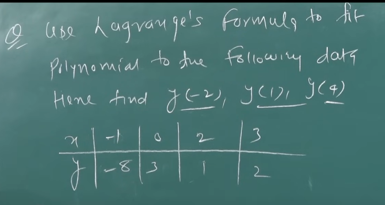
Let’s create the pairings of the data first.

$(x_0,y_0)=(-1,-8)$

$(x_1,y_1)=(0,3)$

$(x_2,y_2)=(2,1)$

$(x_3,y_3)=(3,2)$

So, $L_0=\frac{(x-0)(x-2)(x-3)}{(-1-0)(-1-2)(-1-3)}\times -8=\frac{2(x-0)(x-2)(x-3)}{3}$

$L_1=\frac{(x+1)(x-2)(x-3)}{(0+1)(0-2)(0-3)}\times 3=\frac{(x+1)(x-2)(x-3)}{2}$

$L_2=\frac{(x+1)(x-0)(x-3)}{(2+1)(2-0)(2-3)}\times 1=\frac{(x+1)(x-0)(x-3)}{(-6)}$

$L_3=\frac{(x+1)(x-0)(x-2)}{(3+1)(3-0)(3-2)}\times 2=\frac{(x+1)(x-0)(x-2)}{6}$

For $y(-2)$ :

$\frac{2(-2-0)(-2-2)(-2-3)}{3}+\frac{(-2+1)(-2-2)(-2-3)}{2}+\frac{(-2+1)(-2-0)(-2-3)}{-6}$

$+\frac{(-2+1)(-2-0)(-2-2)}{6}$

$=\frac{(-4)(-4)(-5)}{3}+\frac{(-1)(-4)(-5)}{2}+\frac{(-1)(-2)(-5)}{-6}+\frac{(-1)(-2)(-4)}{6}$

$=\frac{-80}{3}-\frac{20}{2}+\frac{-10}{-6}+\frac{-8}{6}$

$=\frac{-80}{3}-\frac{10}{1}+\frac{5}{3}+\frac{-4}{3}$

$=\frac{-10}{1}+\frac{-79}{3}=\frac{-30-79}{3}=\frac{-109}{3}\approx \boxed{-36.333}$

Now in a similar manner, we can find the values of $y(1)$ and $y(4)$ as:

---

3. Newton’s Divided Difference interpolation

Newton’s Divided Difference formula is used to find a polynomial that passes through a given set of points:

$(x_0,y_0),(x_1,y_1),(x_2,y_2),...,(x_n,y_n)$

It builds the interpolating polynomial in a way that doesn’t require equally spaced x-values — unlike Newton’s Forward/Backward Difference, which assumes the x-values are evenly spaced.

Building the difference table.

Unlike Newton’s forward and backward interpolation which use the same difference table, the divided difference has a different type of table.

The process uses a table, and it’s all about recursive differences.
For each pair of values, you compute:

First-order divided difference:

$f[x_0,x_1]=\frac{f(x_1)-f(x_0)}{x_1-x_0}$​

Second-order divided difference:

$f[x_0,x_1,x_2]=\frac{f[x_1,x_2]-f[x_0,x_1]}{x_2-x_0}$​

Third-order divided difference:

$f[x_0,x_1,x_2,x_3]=\frac{f[x_1,x_2,x_3]-f[x_0,x_1,x_2]}{x_3-x_0}$​

…and so on.

---

The Final Polynomial:

Once you’ve got the divided differences, the interpolating polynomial looks like this:

$P(x)=f(x_0)+(x-x_0)\Delta f(x_0)+(x-x_0)(x-x_1){\Delta }^{2}f(x_0)+\dots$

Each new term:

• adds another factor of $(x-x_k)$,

• and multiplies it by the corresponding divided difference.

---

💡 Why is it Efficient?

• You can add new points without re-computing the whole polynomial.

• It doesn’t assume any uniformity in x-values.

• Computationally lighter than solving a whole system of linear equations (like with Lagrange).

---

Example 1.

https://www.youtube.com/watch?v=zdyUwzOm1zw&list=PLU6SqdYcYsfLrTna7UuaVfGZYkNo0cpVC&index=4

So we have the first example from the Lagrange’s Interpolation problem.

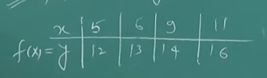
Let’s start with building the table :

$x$	$f(x)$	$\Delta f(x)$	${\Delta }^{2}f(x)$	${\Delta }^{3}f(x)$
5	12
		$\frac{13-12}{6-5}=1$
6	13		$\frac{\frac{1}{3}-1}{9-5}=-\frac{1}{6}$
		$\frac{14-13}{9-6}=\frac{1}{3}$		$\frac{1}{20}$
9	14		$\frac{1-\frac{1}{3}}{11-6}=\frac{2}{15}$
		$\frac{16-14}{11-9}=1$
11	16

Now we can simply apply the values from the table in the formula as

$P(x)=12+(x-5)(1)+(x-5)(x-6)(-\frac{1}{6})+(x-5)(x-6)(x-9)(\frac{1}{20})$

Now, for $x=10$

$⟹P(10)=12+(10-5)(1)+(10-5)(10-6)(-\frac{1}{6})+(10-5)(10-6)(10-9)(\frac{1}{20})$

$⟹P(10)=12+5-\frac{10}{3}+1$

$⟹P(10)=18-\frac{10}{3}$

$⟹P(10)\approx 14.667$

So we get the same answer using Newton’s divided difference method as well.

---