Numerical Methods -- Integration -- Module 3

---

Index

1. Numerical Integration
2. 1. The Trapezoidal Rule of Numerical Integration
3. 2. Simpson’s 1/3 rule
4. Solved Examples

---

Numerical Integration

Overview of Numerical Integration

Numerical integration methods allow us to estimate the area under a curve, that is, the integral of a function, using discrete data points. The two most common techniques are:

• Trapezoidal Rule

• Simpson’s 1/3 Rule

Each method has its own advantages, assumptions, and error characteristics.

---

https://www.youtube.com/watch?v=iviiGB5vxLA&list=PLU6SqdYcYsfLrTna7UuaVfGZYkNo0cpVC&index=5

Suppose we have a definite integral like this:

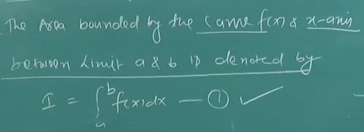
Now suppose this is the area defined by this integral

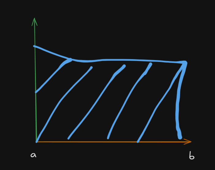
To solve this, we can divide the interval (a,b) into n-equal intervals of length $h$ , which is called the step-size.

Now depending on how the interval (a,b) is divided, there are two rules which can be applied to solve the integral.

1. The Trapezoidal Rule of Numerical Integration

Concept

The trapezoidal rule approximates the area under a curve by dividing it into a series of trapezoids rather than rectangles. The area of each trapezoid is computed and summed up.

For a function $f(x)$ on the interval $[a,b]$ divided into $n$ equal subintervals of width $h=\frac{b-a}{n}$​, the composite trapezoidal rule is:

${\int }_a^{b}f(x)dx\approx \frac{h}{2}[f(x_0)+2f(x_1)+2f(x_2)+\cdots +2f(x_{n-1})+f(x_n)]$

Do note that the end points don’t have any coefficients so $x_0$ and $x_n$ don’t have any coefficients attached.

or

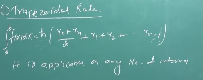
where $y_0$ and $y_n$ are the first and last terms respectively, followed by the remaining terms.

Error Estimate

The error $E_T$​ for the trapezoidal rule is given by:

$E_T=-\frac{(b-a)h^2}{12}{f}^{\prime \prime }(\xi )$,

for some $\xi \in [a,b]$. The error depends on the second derivative of $f(x)$; if $f(x)$ is nearly linear, the error will be small.

---

2. Simpson’s 1/3 rule

Concept

Simpson’s 1/3 rule approximates the area under the curve by fitting quadratic polynomials (parabolas) to the function over pairs of subintervals. It provides better accuracy than the trapezoidal rule when the function is smooth.

Requirements

• The number of subintervals $n$ must be even.
• The interval is again $[a,b]$ with $h=\frac{b-a}{n}$

Formula

The composite Simpson’s 1/3 rule is:

${\int }_a^{b}f(x)dx\approx \frac{h}{3}[f(x_0)+4f(x_1)+2f(x_2)+4f(x_3)+\cdots +4f(x_{n-1})+f(x_n)]$

or

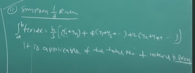
where $y_1$ , $y_3$ are the odd terms and $y_2$ , $y_4$ are the even terms.

This means that 4 is multiplied to the odd terms and 2 is multiplied to the even terms.

Do note that the end points don’t have any coefficients so $y_0$ and $y_n$ don’t have any coefficients attached.

Error Estimate

The error $E_S$ for Simpson’s rule is:

$E_S=\frac{-(b-a)h^4}{180}{f}^{(4)}(\xi )$,

for some $\xi \in [a,b]$. Notice the higher power of $h$ in the error term, which explains why Simpson’s rule is generally more accurate for smooth functions.

---

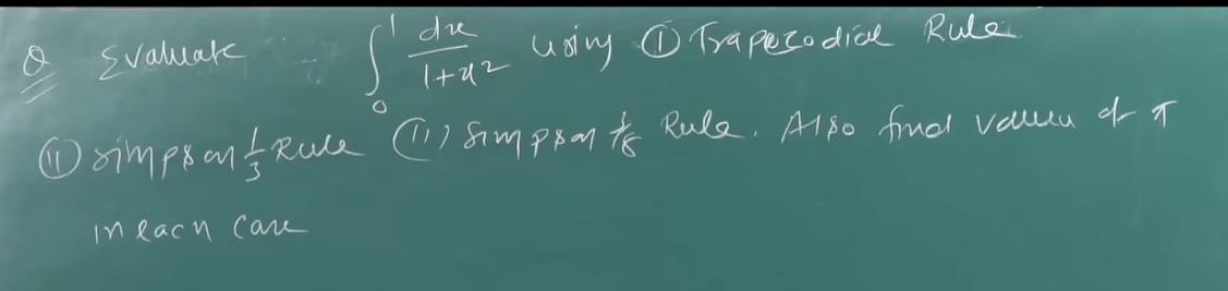
Solved Examples

Let’s go through a simple example to illustrate these methods.

Example 1

Approximate ${\int }_0^2(x^3+x)dx$

with $n=4$ subintervals.

Before trying out any rule, we first find a few data points.

1. Find h

$h=\frac{2-0}{4}=\frac{1}{2}=0.5$

2. Calculate $x_i$ values

Since the step-size is of $0.5$ then for 4 subintervals :

$x_0=0$

$x_1=0+h=0.5$

$x_2=0+2h=1$

$x_3=0+3h=1.5$

$x_4=0+4h=2.0$

3. Evaluate the values for f

1. $f(0)=0^3+0=0$
2. $f(0.5)=0.5^3+0.5=0.625$
3. $f(1.0)=1^3+1=2$
4. $f(1.5)=1.5^3+1.5=4.875$
5. $f(2.0)=2^3+2=10$

Now, we will solve this integral using both the rules.

1. Trapezoidal rule solving

${\int }_0^2(x^3+x)dx\approx \frac{h}{2}[f(x_0)+2f(x_1)+2f(x_2)+2f(x_3)+f(x_4)]$

$=\frac{0.5}{2}[0+2\times 0.625+2\times 2+2\times 4.875+10]$

$=0.25[1.25+4+9.75+10]$

$=0.25[25]$

$=6.25$

2. Simpson’s 1/3 rule solving

${\int }_a^{b}f(x)dx\approx \frac{h}{3}[f(x_0)+4f(x_1)+2f(x_2)+4f(x_3)+f(x_4)]$

$=\frac{0.5}{3}[0+4\times 0.625+2\times 2+4\times 4.875+10]$ $=\frac{0.5}{3}[0+2.5+4+19.5+10]$

$=\frac{0.5}{3}\times 36$

$=0.5\times 12$

$=6.0$

Comparison

• Trapezoidal Rule: $6.25$

• Simpson’s 1/3 Rule: $6$

Depending on the function’s curvature, Simpson’s rule often gives a better approximation. In this case, Simpson’s 1/3 rule approximates the integral as $6$.

---

Example 2

We are not going to do the 3/8 rule as it’s not in our syllabus.

So we have :

${\int }_0^1\frac{dx}{1+x^2}$

Let’s solve this for 6 sub intervals ($n=6$)

So firstly we will find the value of $h$

$h=\frac{1-0}{6}=\frac{1}{6}=0.16667$

So with a step size of $0.16667$,

$x_0=0$

$x_1=0+h=0.16667$

$x_2=0+2h=0.33333$

$x_3=0+3h=0.50001$

$x_4=0+4h=0.66667$

$x_5=0+5h=0.83333$

$x_6=0+6h=1$

Now we find the values of $f(x_0)$ till $f(x_6)$

1. $f(0)=\frac{1}{1+0^2}=1$

2. $f(0.16667)=\frac{1}{1+0.16667^2}\approx \frac{1}{1.02778}\approx 0.97297$

3. $f(0.33333)=\frac{1}{1+0.33333^2}\approx \frac{1}{1.11111}\approx 0.9$

4. $f(0.50001)=\frac{1}{1+0.50001^2}\approx \frac{1}{1.25001}\approx 0.8$

5. $f(0.66667)=\frac{1}{1+0.66667^2}\approx \frac{1}{1.44444}\approx 0.6923$

6. $f(0.83333)=\frac{1}{1+0.83333^2}\approx \frac{1}{1.69444}\approx 0.5909$

7. $f(1)=\frac{1}{1+1^2}=\frac{1}{2}=0.5$

---

1. Solving using Trapezoidal Rule

${\int }_0^2(\frac{1}{1+x^2})dx\approx \frac{h}{2}[f(x_0)+2f(x_1)+2f(x_2)+2f(x_3)+2f(x_4)+2f(x_5)+f(x_6)]$

$=\frac{0.16667}{2}[1+1.94594+1.8+1.6+1.3846+1.1818+0.5]$

$=\frac{0.16667\times 9.41234}{2}$ $=\frac{1.568754708}{2}$

$\approx 0.784377353$

2. Solving using Simpson’s 1/3 rule.

${\int }_0^2(\frac{1}{1+x^2})dx\approx \frac{h}{3}[f(x_0)+4f(x_1)+2f(x_2)+4f(x_3)+2f(x_4)+4f(x_5)+f(x_6)]$

$=\frac{0.16667}{3}[1+3.89188+1.8+3.2+1.3846+2.3636+0.5]$

$=\frac{0.16667}{3}[14.14008]$

$\approx 0.785575711$

As we can see, Simpson’s 1/3 rule resulted in a better precision than the trapezoidal rule.

---